cherab.inversion.tools.Derivative
-
class cherab.inversion.tools.Derivative(grid, grid_map=
None)Source¶ Bases:
objectClass for derivative matrices.
This class is used to generate various derivative matrices using grid coordinates information.
Derivative matrices are applied to spatial profiles defined on the grid coordinates (cartesian, cylindrical, etc.) and are created with their grid coordinates.
- Parameters:
- grid : (..., L, M, ndim) or (N, ), array_like
The grid coordinates. The shape of the array means the resolution of the grid. For example, in 3-D spatial grid, the shape is (L, M, N, 3), where 3 is the dimension of the grid. If the grid is 1-D like (N,), it is automatically reshaped to (N, 1).
- grid_map : (..., L, M) array_like, optional
The map of the grid index with
inttype. The shape of the array must be the same as the grid shape except for the last dimension. The masked area is represented by negative values. If None, the grid_map is automatically created by the order of the grid array.
Examples
>>> import numpy as np
>>> from cherab.inversion import Derivative
>>> x = np.linspace(-10, 10, 21)
>>> derivative = Derivative(x)
>>> derivative
Derivative(grid=array(21, 1), grid_map=array(21,))
Methods
matrix_along_axis(axis[, diff_type, boundary])Generate derivative matrix along the specified axis.
matrix_gradient(func[, diagonal])Criate derivative matrices based on the gradient of the given function.
Attributes
The grid coordinates.
The map of the grid index.
-
matrix_along_axis(axis: int, diff_type: 'forward' | 'backward' =
'forward', boundary: 'dirichlet' | 'neumann' | 'periodic' ='dirichlet') csr_arraySource¶ Generate derivative matrix along the specified axis.
Note
If the grid has masked area, edges before the masked area take either the dirichlet (forward) or neumann (backward) condition. The periodic boundary condition is only available for the last and first points along the axis.
- Parameters:
- axis: int
The axis to calculate the derivative matrix. The axis must be in the grid dimensions.
- diff_type: 'forward' | 'backward' =
'forward'¶ The type of the difference method, by default “forward”.
- boundary: 'dirichlet' | 'neumann' | 'periodic' =
'dirichlet'¶ The boundary condition of the derivative matrix, by default “dirichlet”. If the boundary condition is “dirichlet”, the outer boundary is set to zero. If the boundary condition is “neumann”, the difference type is set to the opposite direction at the edge of the grid. If the boundary condition is “periodic”, the first and last points are connected.
- Returns:
csr_array – The derivative matrix along the specified axis.
- Raises:
ValueError – If
axisis invalid,diff_typeis not one of “forward” or “backward”, orboundaryis not one of “dirichlet”, “neumann”, or “periodic”.
Examples
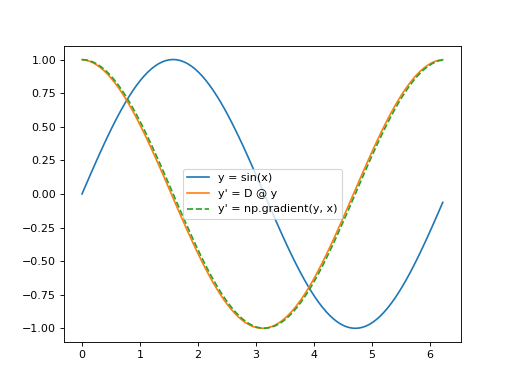
Firstly, let us operate the derivative matrix to a simple 1-D profile and compare it with gradient values calculated by the
numpy.gradientfunction.import numpy as np import matplotlib.pyplot as plt from cherab.inversion import Derivative # Create a sample 1-D sine profile x = np.linspace(0, 2 * np.pi, 100, endpoint=False) y = np.sin(x) # Calculate the derivative matrix derivative = Derivative(x) dmat = derivative.matrix_along_axis(0, boundary="dirichlet") # Compare gradient values plt.plot(x, y, label="y = sin(x)") plt.plot(x, dmat @ y, label="y' = D @ y") plt.plot(x, np.gradient(y, x), label="y' = np.gradient(y, x)", linestyle="--") plt.legend() plt.show()(
Source code,png,hires.png,pdf)
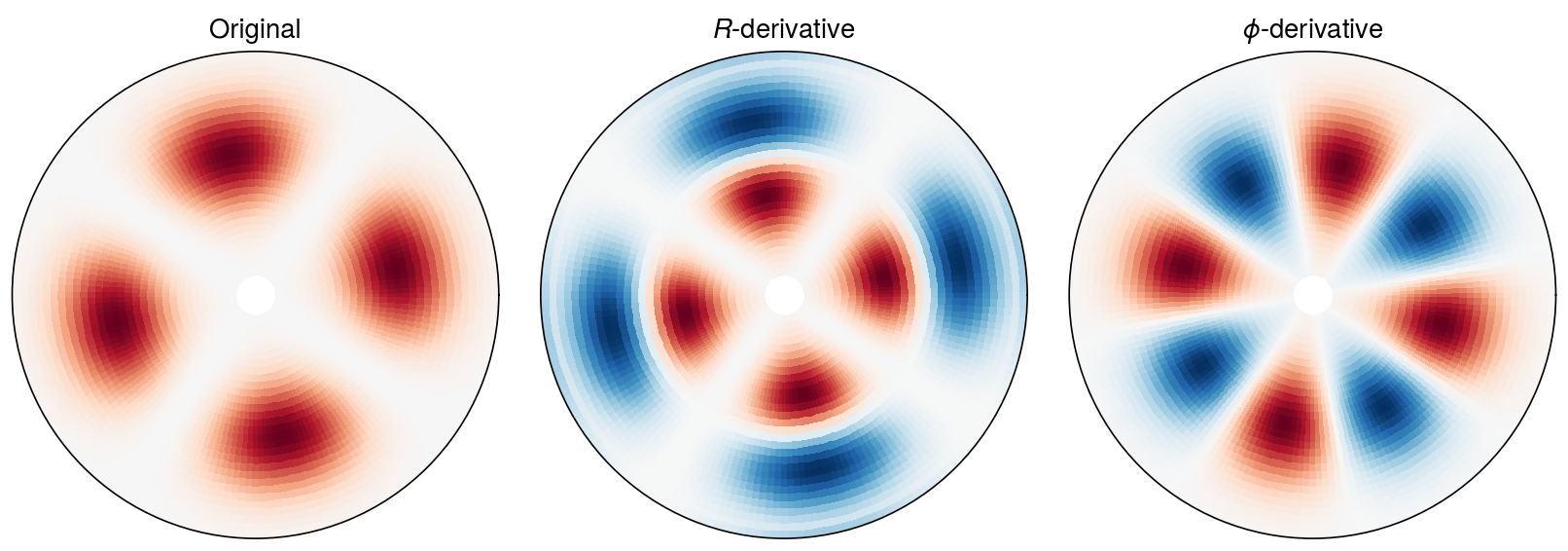
Next, we create a sample 2-D profile in cylindrical coordinates and apply the derivative along the R and Phi axis to the profile.
import numpy as np
import ultraplot as uplt

from cherab.inversion import Derivative

# R-Phi grids
radius = np.linspace(0.1, 1, 30)
angles = np.linspace(0, 2 * np.pi, 180, endpoint=False)

# Create voxels center coordinates in (x, y, z)
rr, pp = np.meshgrid(radius, angles)
centers = np.zeros((30, 180, 1, 3))
centers[:, :, 0, 0] = (rr * np.cos(pp)).T
centers[:, :, 0, 1] = (rr * np.sin(pp)).T
centers[:, :, 0, 2] = 0

# Create a 2-D profile
indices = np.ndindex(centers.shape[:3])
profile = np.zeros(centers.shape[:3])

CENTER = 0.6
WIDTH = 0.05
PHASE = -np.pi / 4
for ir, ip, iz in indices:
    profile[ir, ip, iz] = (1 + np.cos(angles[ip] * 4 + PHASE)) * np.exp(
        -((radius[ir] - CENTER) ** 2) / WIDTH
    )


# Operate derivative
deriv = Derivative(
    centers,
    np.arange(np.prod(centers.shape[:3]), dtype=np.int32).reshape(centers.shape[:3]),
)
dmat_r = deriv.matrix_along_axis(0, diff_type="forward", boundary="dirichlet")
dmat_p = deriv.matrix_along_axis(1, diff_type="forward", boundary="periodic")

profile_dr = dmat_r @ profile.ravel()
profile_dp = dmat_p @ profile.ravel()
profile_dr = profile_dr.reshape(centers.shape[:3])
profile_dp = profile_dp.reshape(centers.shape[:3])

# Plot the profiles
fig, axes = uplt.subplots(ncols=3, proj="polar")
for ax, f, title in zip(
    axes,
    [profile, profile_dr, profile_dp],
    ["Original", "$R$-derivative", "$\\phi$-derivative"],
    strict=True,
):
    vmax = np.max(np.abs(f))
    ax.pcolormesh(
        angles,
        radius,
        f[..., 0],
        vmax=vmax,
        vmin=-vmax,
        discrete=False,
    )
    ax.format(title=title)

axes.format(
    grid=False,
    rformatter="null",
    thetaformatter="null",
)

fig.show()
(
Source code,png,hires.png,pdf)
-
matrix_gradient(func: Callable[[float, float], float], diagonal: bool =
False) tuple[csr_array, csr_array]Source¶ Criate derivative matrices based on the gradient of the given function.
This function returns derivative matrices along the parallel and perpendicular directions to the gradient of the given function. The gradient is calculated by the finite central difference using
numpy.gradientat each grid point.Warning
Currently, this method can only be used for a 2-D function, which uses the first and second axis of the grid coordinates, i.e. the grid shape is only allowed to be
(L, M, ndim)or(L, M, N, ndim). and the function use theLandMas the first and second axis respectively.- Parameters:
- Returns:
dmat_parallel (
csr_array) – The derivative matrix along the parallel direction to the gradient.dmat_perpendicular (
csr_array) – The derivative matrix along the perpendicular direction to the gradient.
- Raises:
ValueError – If the grid shape is invalid for this method.
NotImplementedError – If the grid shape or coordinate dimension is over 3-D.
Examples
Let us create a sample 2-D profile and apply the derivative matrices along the parallel and perpendicular directions to the gradient of the concentrically monotonically increasing function.
import numpy as np
import ultraplot as uplt

from cherab.inversion import Derivative

# X-Y grids
x = np.linspace(-1, 1, 60)
y = np.linspace(-1, 1, 60)

# Create voxels center coordinates in (x, y, z)
xx, yy = np.meshgrid(x, y)
centers = np.zeros((x.size, y.size, 1, 3))
centers[:, :, 0, 0] = xx.T
centers[:, :, 0, 1] = yy.T
centers[:, :, 0, 2] = 0

# Create a 2-D profile
indices = np.ndindex(centers.shape[:3])
profile = np.zeros(centers.shape[:3])

CENTER = 0.6
WIDTH = 0.05
PHASE = -np.pi / 4

profile = np.zeros(centers.shape[:3])
radius = np.hypot(xx, yy).T
angles = np.arctan2(yy, xx).T
profile[..., 0] = (1 + np.cos(angles * 4 + PHASE)) * np.exp(-((radius - CENTER) ** 2) / WIDTH)


def scalar_func(x, y):
    """Scalar function to be used in the derivative calculation."""
    return np.hypot(x, y)


# Operate derivative
deriv = Derivative(centers)
dmat_para, dmat_perp = deriv.matrix_gradient(scalar_func)
profile_para = dmat_para @ profile[deriv.grid_map > -1]
profile_perp = dmat_perp @ profile[deriv.grid_map > -1]
profile_para = profile_para.reshape(deriv.grid_map.shape)
profile_perp = profile_perp.reshape(deriv.grid_map.shape)

# Calculate Scalar function values and its gradient
fvals = scalar_func(xx, yy)
grads = np.gradient(fvals, centers[:, 0, 0, 0], centers[0, :, 0, 1])

# Calculate the gradient of the profile
grad_profile = np.gradient(profile[..., 0], centers[:, 0, 0, 0], centers[0, :, 0, 1])
grad_profile = np.hypot(grad_profile[0], grad_profile[1])[:, :, None]

# Plot the profiles
fig, axes = uplt.subplots(nrows=2, ncols=3)
for ax, f, title in zip(
    axes,
    [
        fvals[..., np.newaxis],
        [grads[0], grads[1]],
        [-grads[1], grads[0]],
        profile,
        profile_para,
        profile_perp,
    ],
    [
        "$f(x, y)$",
        "$\\nabla f(x, y)$",
        "Perp of $\\nabla f(x, y)$",
        "Profile",
        "$\\nabla_\\parallel$-derivative",
        "$\\nabla_\\perp$-derivative",
    ],
    strict=False,
):
    if "\\nabla f(x, y)" not in title:
        ax.pcolormesh(
            centers[:, 0, 0, 0],
            centers[0, :, 0, 1],
            f[..., 0].T,
            discrete=False,
            vmax=np.max(np.abs(f)),
            vmin=-np.max(np.abs(f)),
        )
    else:
        ax.quiver(
            centers[:, 0, 0, 0][::8],
            centers[0, :, 0, 1][::8],
            f[0][::8, ::8].T,
            f[1][::8, ::8].T,
            scale=10,
        )
    ax.format(title=title)

axes.format(
    aspect="equal",
    xlabel="X",
    ylabel="Y",
    tickdir="in",
)

fig.show()
(
Source code,png,hires.png,pdf)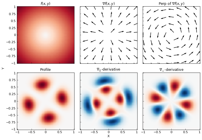