Minimum Fisher Regularization (MFR) tomography
This page shows how to apply the MFR method to the specific case of tomography.
The basic theory of the MFR is described in this page.
Example Tomography Problem
As the example tomography problem, we consider the bolometer measurement and use the geometry matrix calculated at cherab.core documentation.
[1]:
import pickle
from pathlib import Path
from pprint import pprint

import numpy as np
import ultraplot as uplt

from cherab.inversion import MFR
from cherab.inversion.data import get_sample_data
from cherab.inversion.tools import derivative_matrix

# path to the directory to store the MFR results
store_dir = Path().cwd() / "01-mfr"
store_dir.mkdir(exist_ok=True)
The sample data can be retrieved by get_sample_data function with "bolo.npz" argument.
[2]:
# Load the sample data
grid_data = get_sample_data("bolo.npz")

# Extract the data having several keys
grid_centres = grid_data["grid_centres"]
voxel_map = grid_data["voxel_map"].squeeze()
mask = grid_data["mask"].squeeze()
gmat = grid_data["sensitivity_matrix"]

# Extract grid limits
dr = grid_centres[1, 0, 0] - grid_centres[0, 0, 0]
dz = grid_centres[0, 1, 1] - grid_centres[0, 0, 1]
rmin, rmax = grid_centres[0, 0, 0] - 0.5 * dr, grid_centres[-1, 0, 0] + 0.5 * dr
zmin, zmax = grid_centres[0, 0, 1] - 0.5 * dz, grid_centres[0, -1, 1] + 0.5 * dz

print(f"{grid_centres.shape = }")
print(f"{voxel_map.shape = }")
print(f"{mask.shape = }")
print(f"{gmat.shape = }")
print(f"gmat density: {np.count_nonzero(gmat) / gmat.size:.2%}")
grid_centres.shape = (40, 60, 2)
voxel_map.shape = (40, 60)
mask.shape = (40, 60)
gmat.shape = (48, 1210)
gmat density: 8.35%
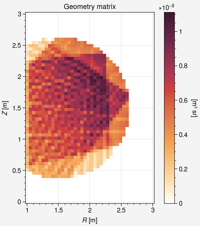
The geometry matrix density is 8.35% so this problem is known as the sparse problem as well.
Show the geometry matrix
[3]:
sensitivity_2d = np.full(voxel_map.shape, np.nan)
sensitivity_2d[mask] = gmat.sum(axis=0)

fig, ax = uplt.subplots()
image = ax.imshow(
    sensitivity_2d.T,
    origin="lower",
    extent=(rmin, rmax, zmin, zmax),
    colorbar="r",
    colorbar_kw=dict(label="[m³ sr]"),
)
ax.format(
    xlabel="$R$ [m]",
    ylabel="$Z$ [m]",
    title="Geometry matrix",
)
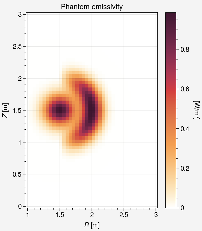
Define phantom emission profile
As a test emission profile, we define the following phantom emission profile which is used in the cherab.core documentation as well.
[4]:
PLASMA_AXIS = np.array([1.5, 1.5])
LCFS_RADIUS = 1
RING_RADIUS = 0.5

RADIATION_PEAK = 1
CENTRE_PEAK_WIDTH = 0.05
RING_WIDTH = 0.025


def emission_function_2d(rz_point: np.ndarray) -> float:
    direction = rz_point - PLASMA_AXIS
    bearing = np.arctan2(direction[1], direction[0])

    # calculate radius of coordinate from magnetic axis
    radius_from_axis = np.hypot(*direction)
    closest_ring_point = PLASMA_AXIS + (0.5 * direction / radius_from_axis)
    radius_from_ring = np.hypot(*(rz_point - closest_ring_point))

    # evaluate pedestal -> core function
    if radius_from_axis <= LCFS_RADIUS:
        central_radiatior = RADIATION_PEAK * np.exp(-(radius_from_axis**2) / CENTRE_PEAK_WIDTH)

        ring_radiator = (
            RADIATION_PEAK * np.cos(bearing) * np.exp(-(radius_from_ring**2) / RING_WIDTH)
        )
        ring_radiator = max(0, ring_radiator)

        return central_radiatior + ring_radiator
    else:
        return 0


# Create a phantom vector
phantom = np.zeros(gmat.shape[1])

nr, nz = voxel_map.shape
for ir, iz in np.ndindex(nr, nz):
    index = voxel_map[ir, iz]
    if index < 0:
        continue
    phantom[index] = emission_function_2d(grid_centres[ir, iz])

# Create a 2D phantom
phantom_2d = np.full(voxel_map.shape, np.nan)
phantom_2d[mask] = phantom
[5]:
fig, ax = uplt.subplots()
image = ax.imshow(
    phantom_2d.T,
    origin="lower",
    extent=(rmin, rmax, zmin, zmax),
    colorbar="r",
    colorbar_kw=dict(label="[W/m³]"),
)
ax.format(
    title="Phantom emissivity",
    xlabel="$R$ [m]",
    ylabel="$Z$ [m]",
)
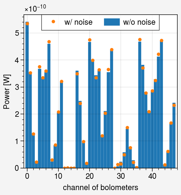
Compute the measurement data
The bolometer measurement data should be calculated by the ray-tracing method however, we generate the measurement data by the multiplication of the geometry matrix and the phantom profile. As the noise, we add the Gaussian noise with the standard deviation of 1% of the maximum value of the measurement data.
[6]:
gmat /= 4.0 * np.pi  # Divide by 4π steradians to use for measuring power in [W].

data = gmat @ phantom

rng = np.random.default_rng()
data_w_noise = data + rng.normal(0, data.max() * 1.0e-2, data.size)
data_w_noise = np.clip(data_w_noise, 0, None)
[7]:
fig, ax = uplt.subplots()
ax.bar(np.arange(data.size), data, label="w/o noise")
ax.plot(data_w_noise, ".", c="C1", label="w/ noise")
ax.legend()
ax.format(
    xlabel="channel of bolometers",
    ylabel="Power [W]",
    xlim=(-1, data.size),
)
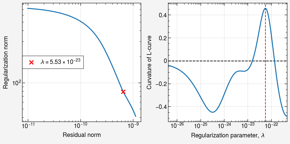
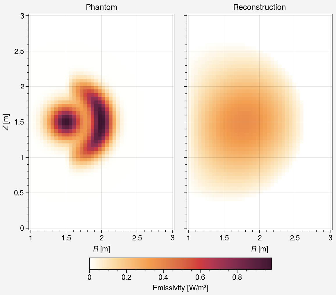
1. Solve by the Laplacian regularization
The Laplacian regularization (or Phillips regularization(Phillips 1962)) is one of the most popular regularization methods. However, this regularization tends to over-smooth the solution, which is unsuitable for the sparse problem. Let’s look at this behavior by solving the tomography problem with the laplacian regularization. As the optimization method, we use the L-curve method.
[8]:
from cherab.inversion import SVD, Lcurve
from cherab.inversion.tools import laplacian_matrix

lmat = laplacian_matrix(voxel_map.shape, (dr, dz), mask=mask)

svd = SVD(gmat, H=lmat.T @ lmat, data=data_w_noise)
lcurve = Lcurve()
sol, status = svd.solve(lcurve)

# Plot criteria
fig, axes = uplt.subplots(ncols=2, share=False)
lcurve.plot_L_curve(axes=axes[0])
lcurve.plot_curvature(axes=axes[1])
axes[0].format(
    yformatter="log",
)
axes.format(
    xformatter="log",
)
Comparison of the solution with the phantom reveals over-smoothing, resulting in lost details of the phantom.
[9]:
vmin = min(sol.min(), phantom.min())
vmax = max(sol.max(), phantom.max())

fig, axes = uplt.subplots(ncols=2, spanx=False)
for ax, value, label in zip(
    axes,
    [phantom, sol],
    ["Phantom", "Reconstruction"],
    strict=True,
):
    image = np.full(voxel_map.shape, np.nan)
    image[mask] = value

    im = ax.imshow(
        image.T,
        origin="lower",
        extent=(rmin, rmax, zmin, zmax),
        vmin=vmin,
        vmax=vmax,
    )
    ax.format(
        title=label,
    )

fig.colorbar(
    im,
    ax=axes,
    loc="b",
    shrink=0.6,
    label="Emissivity [W/m³]",
)

axes.format(
    xlabel="$R$ [m]",
    ylabel="$Z$ [m]",
)
Quantitative evaluation
Let’s assess the solution quantitatively using the relative error, total power, and negative power values. Each value is calculated as follows:
where \(\mathbf{x}_\mathrm{recon}\) and \(\mathbf{x}_\mathrm{phan}\) are the reconstructed and phantom profiles, respectively. \(\mathbf{x}_i\) represents the \(i\)-th element of the profile, and \(v_i\) is the volume of the \(i\)-th voxel calculated with the Pappus theorem:
where \(\Delta r\) and \(\Delta z\) are the radial and vertical voxel sizes, respectively, and \(r_i\) is the radial position of the \(i\)-th voxel.
[10]:
volumes = dr * dz * 2.0 * np.pi * grid_centres[:, :, 0]
volumes = volumes[mask]

print(
    "The relative error           :",
    f"{np.linalg.norm(sol - phantom) / np.linalg.norm(phantom):.2%}",
)
print("--------------------------------------------")
print(f"total power of phantom       : {phantom @ volumes:.4g} W")
print(f"total power of reconstruction: {sol @ volumes:.4g} W")
print(f"total negative power of reconstruction: {sol[sol < 0] @ volumes[sol < 0]:.4g} W")
The relative error           : 60.51%
--------------------------------------------
total power of phantom       : 4.848 W
total power of reconstruction: 5.049 W
total negative power of reconstruction: 0 W
2. Solve by the MFR regularization
Prepare the derivative matrices
Before performing the MFR tomography, we need to create derivative matrices. Here \(\mathbf{H}\) is defined as follows:
where \(\mathbf{D}_r\) and \(\mathbf{D}_z\) are derivative matrices along the \(r\) and \(z\) coordinate direction, respectively.
[11]:
dmat_r = derivative_matrix(voxel_map.shape, dr, axis=0, scheme="forward", mask=mask)
dmat_z = derivative_matrix(voxel_map.shape, dz, axis=1, scheme="forward", mask=mask)

dmat_pair = [(dmat_r, dmat_r), (dmat_z, dmat_z)]
pprint(dmat_pair)
[(<Compressed Sparse Column sparse array of dtype 'float64'
        with 2376 stored elements and shape (1210, 1210)>,
  <Compressed Sparse Column sparse array of dtype 'float64'
        with 2376 stored elements and shape (1210, 1210)>),
 (<Compressed Sparse Column sparse array of dtype 'float64'
        with 2388 stored elements and shape (1210, 1210)>,
  <Compressed Sparse Column sparse array of dtype 'float64'
        with 2388 stored elements and shape (1210, 1210)>)]
Reconstruct
Let us do the MFR tomography. cherab.inversion offers the MFR class and simple solve method.
The store_regularizers parameter of the solve method stores the regularizer object Lcurve instance at each MFR iteration.
[12]:
num_mfi = 4  # number of MFR iterations
eps = 1.0e-6  # small positive number to avoid division by zero
tol = 1.0e-3  # tolerance for the convergence criterion

mfr = MFR(gmat, dmat_pair, data=data_w_noise)
sol, stats = mfr.solve(
    miter=num_mfi,
    eps=eps,
    tol=tol,
    store_regularizers=True,
    path=store_dir,
)
Evaluate the tomographic reconstruction
Let’s compare the tomographic reconstruction with the phantom profile. We observe that the MFR tomography captures finer details of the phantom profile than the Laplacian regularization.
[13]:
vmin = min(sol.min(), phantom.min())
vmax = max(sol.max(), phantom.max())

fig, axes = uplt.subplots(ncols=2, spanx=False)
for ax, value, label in zip(
    axes,
    [phantom, sol],
    ["Phantom", "Reconstruction"],
    strict=True,
):
    image = np.full(voxel_map.shape, np.nan)
    image[mask] = value

    im = ax.imshow(
        image.T,
        origin="lower",
        extent=(rmin, rmax, zmin, zmax),
        vmin=vmin,
        vmax=vmax,
    )
    ax.format(
        title=label,
    )

fig.colorbar(
    im,
    ax=axes,
    loc="b",
    shrink=0.6,
    label="Emissivity [W/m³]",
)

axes.format(
    xlabel="$R$ [m]",
    ylabel="$Z$ [m]",
)
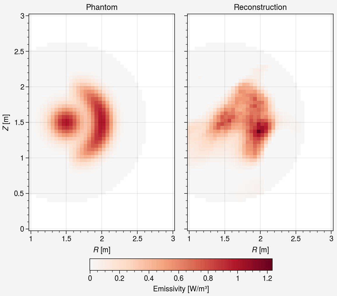
Quantitative evaluations are shown as follows.
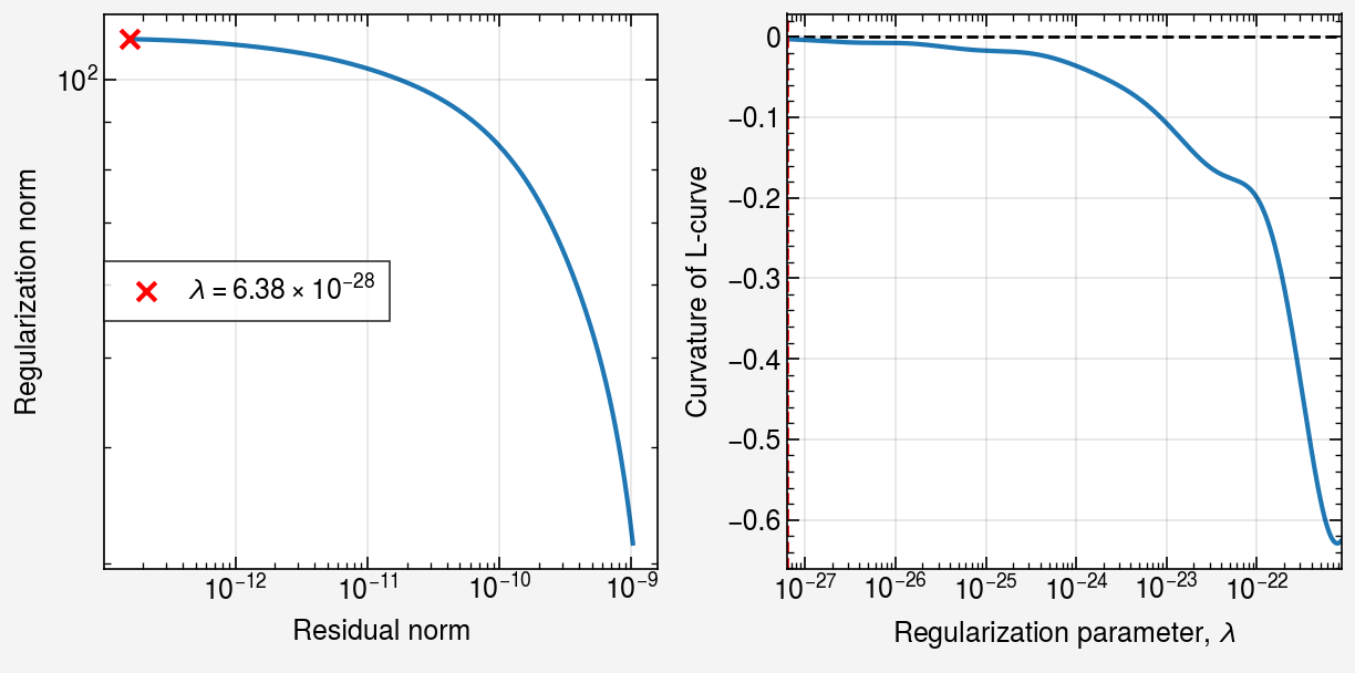
L-curve and its curvature plot
The L-curve of the last solution and its curvature are displayed below.
[14]:
svd = stats["regularizer"]
fig, axes = uplt.subplots(ncols=2, share=False)
lcurve = Lcurve()
lcurve.plot_L_curve(svd, axes=axes[0])
lcurve.plot_curvature(svd, axes=axes[1])
axes[0].format(
    yformatter="log",
)
axes.format(
    xformatter="log",
)
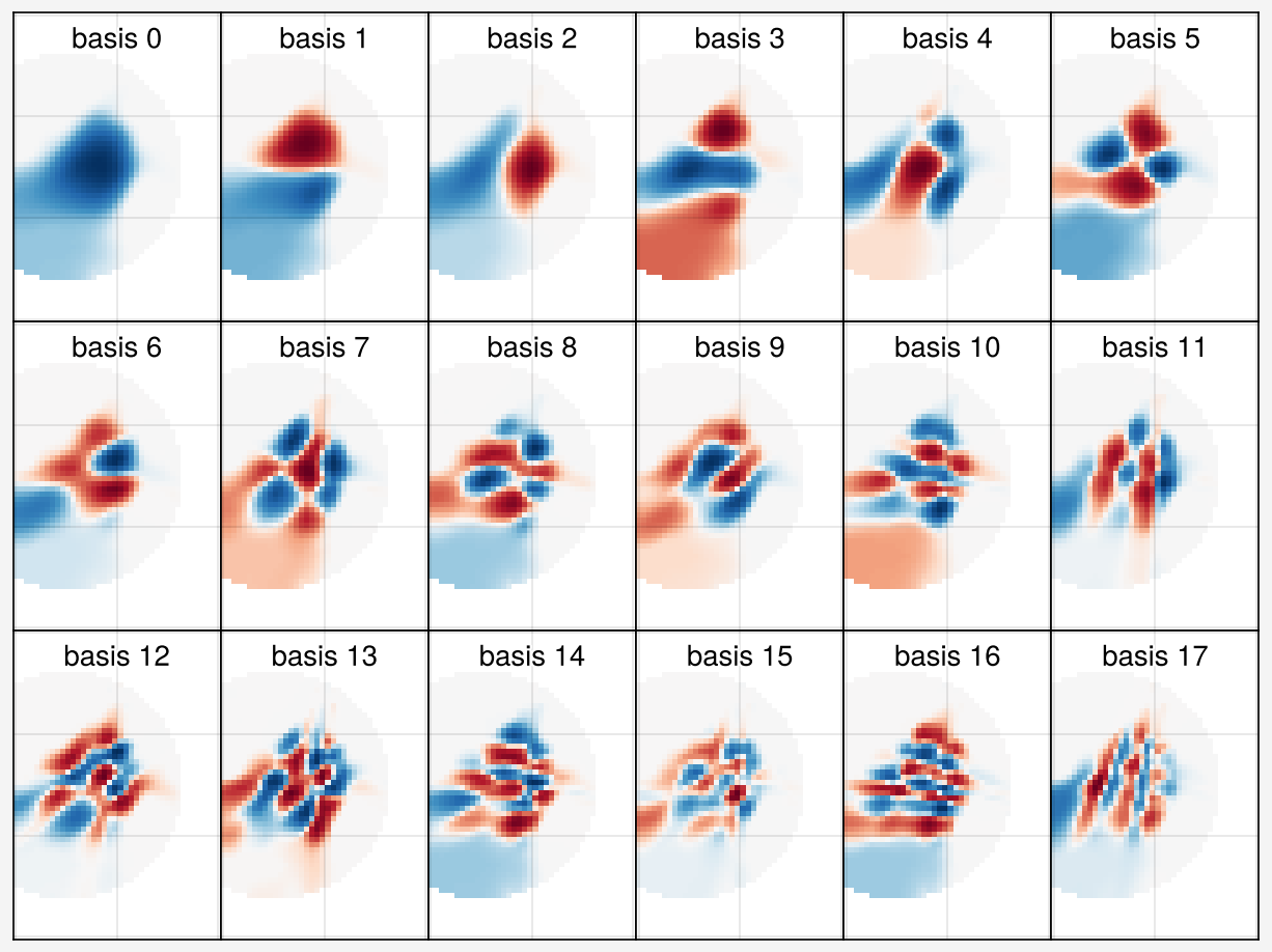
The solution bases from 0-th to 18-th are shown below.
[15]:
from matplotlib.colors import AsinhNorm

fig, axes = uplt.subplots(nrows=3, ncols=6, space=0.0, refwidth=1)

for i, ax in enumerate(axes):
    profile2d = np.full(voxel_map.shape, np.nan)
    profile2d[mask] = svd.basis[:, i]

    absolute = max(abs(svd.basis[:, i].min()), abs(svd.basis[:, i].max()))

    ax.imshow(
        profile2d.T,
        origin="lower",
        extent=(rmin, rmax, zmin, zmax),
        norm=AsinhNorm(vmin=-1 * absolute, vmax=absolute, linear_width=absolute * 1e-1),
    )

    ax.format(
        uctitle=f"basis {i}",
    )

axes.format(
    xtickloc="neither",
    ytickloc="neither",
)
Compare the measurement powers
[16]:
back_calculated_measurements = gmat @ sol

fig, axes = uplt.subplots(
    nrows=2,
    refaspect=2.2,
    refwidth=5,
    sharey=False,
)
ax1, ax2 = axes

# Plot the phantom and the back-calculated measurements
ax1.bar(np.arange(data.size), data, label="Matrix-based measurements")
ax1.plot(back_calculated_measurements, ".", color="C1", label="Back-calculated from inversion")
ax1.legend(ncols=1)
ax1.format(
    ylabel="Power [W]",
)

# Plot the residuals between the measurements b and the back-calculated Tx (b - Tx)
ax2.axhline(0, color="k", linestyle="--")
ax2.bar(np.arange(data.size), data - back_calculated_measurements, color="C2")
ax2.format(
    ylabel="Residual [W]",
)

axes.format(
    xlim=(-1, data.size),
    xlabel="channel of bolometers",
    xlocator=5,
    xminorlocator=1,
)
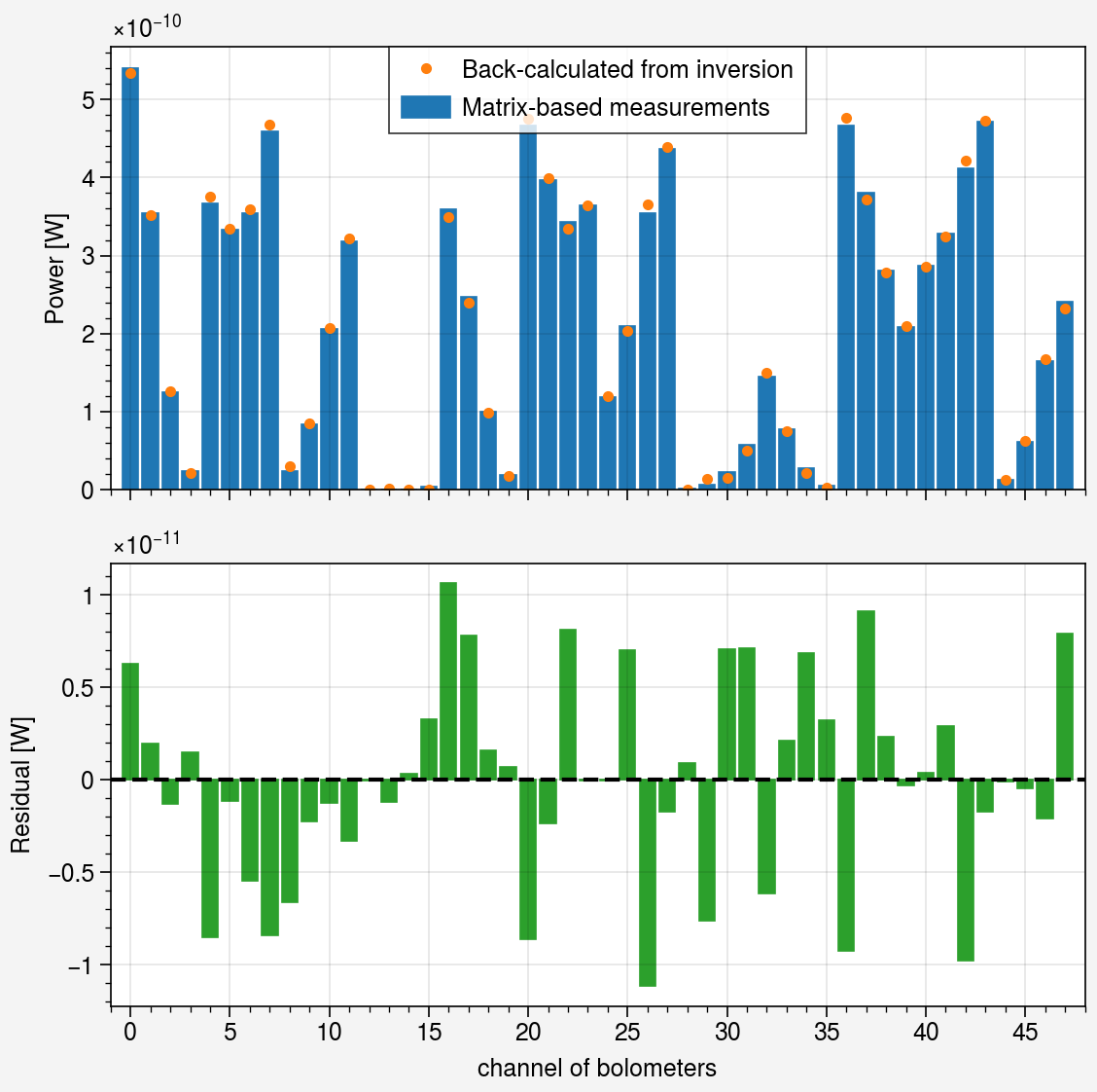
The measured power calculated by multiplying the geometry matrix by the emission vector and the back-calculated power calculated by multiplying the geometry matrix by the inverted emissivity are all in good agreement
[17]:
print(
    "The relative error of power measurements is",
    f"{np.linalg.norm(data - back_calculated_measurements) / np.linalg.norm(data):.2%}",
)
The relative error of power measurements is 1.99%
[18]:
print(
    "The relative error           :",
    f"{np.linalg.norm(sol - phantom) / np.linalg.norm(phantom):.2%}",
)
print("--------------------------------------------")
print(f"total power of phantom       : {phantom @ volumes:.4g} W")
print(f"total power of reconstruction: {sol @ volumes:.4g} W")
print(f"total negative power of reconstruction: {sol[sol < 0] @ volumes[sol < 0]:.4g} W")
The relative error           : 28.48%
--------------------------------------------
total power of phantom       : 4.848 W
total power of reconstruction: 4.883 W
total negative power of reconstruction: -0.002122 W
Iteration history
As described in the MFR definition section, MFR is the iterative method. In order to observe the convergence behavior, we will examine the iteration history.
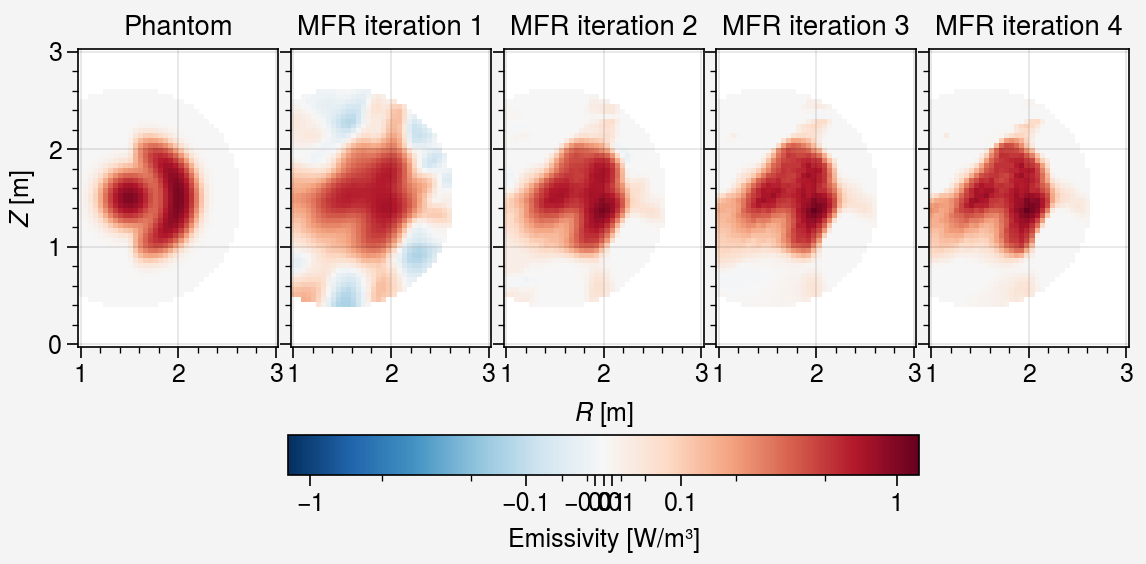
Reconstruction profiles history
Firstly, let us see each iteration solution. To better understand the negative values, we can visualize the solutions using the arcsinh scale.
[19]:
# Stored regularizer files
reg_files = list(store_dir.glob("regularizer_*.pickle"))
reg_files = sorted(reg_files, key=lambda x: int(x.stem.split("_")[-1]))

# Load each solution
sols = []
regs = []
for file in reg_files:
    with open(file, "rb") as f:
        reg = pickle.load(f)

    sols.append(reg.solution(reg.lambda_opt))
    regs.append(reg)

profiles = [phantom] + sols

# set vmin and vmax for all solutions
vmin = min(profile.min() for profile in profiles)
vmax = max(profile.max() for profile in profiles)


# Plot the solutions
fig, axes = uplt.subplots(ncols=len(profiles), wspace=0.5, refwidth=1)

absolute = max(abs(vmax), abs(vmin))
linear_width = absolute * 0.1
norm = AsinhNorm(linear_width=linear_width, vmin=-1 * absolute, vmax=absolute)
i = 0
for ax, profile in zip(axes, profiles, strict=True):
    sol_2d = np.full(voxel_map.shape, np.nan)
    sol_2d[mask] = profile

    im = ax.imshow(
        sol_2d.T,
        origin="lower",
        extent=(rmin, rmax, zmin, zmax),
        norm=norm,
    )
    if i == 0:
        ax.format(title="Phantom")
    else:
        ax.format(title=f"MFR iteration {i}")
    i += 1

fig.colorbar(
    im,
    ax=axes,
    loc="b",
    shrink=0.6,
    label="Emissivity [W/m³]",
)

axes.format(
    xlabel="$R$ [m]",
    ylabel="$Z$ [m]",
)
Quantitative evaluation history
The following plots display the quantitative evaluation changes over the course of the iteration.
[20]:
relative_errors = []
total_powers = []
negative_powers = []

for sol in sols:
    relative_errors.append(np.linalg.norm(sol - phantom) / np.linalg.norm(phantom))
    total_powers.append(sol @ volumes)
    negative_powers.append(sol[sol < 0] @ volumes[sol < 0])

# Append nan value to the last iteration
relative_errors.append(np.nan)
negative_powers.append(np.nan)

# show each value as a bar plot
fig, axes = uplt.subplots(nrows=3, sharey=False, refaspect=2.2, hspace=1)
ax1, ax2, ax3 = axes

x = np.arange(1, len(relative_errors) + 1)  # the label locations
rects = ax1.bar(
    x,
    total_powers + [np.sum(phantom * volumes)],
    color=["C0"] * (len(total_powers)) + ["C1"],
)
ax1.bar_label(rects, padding=-15, fmt="{:.3f}", color="w")
ax1.format(ylabel="Total power [W]")


rects = ax2.bar(x, negative_powers, color="C2")
ax2.bar_label(rects, padding=3, fmt="{:.3f}")
ax2.format(
    ylim=(-0.55, None),
    ylabel="Negative power [W]",
)

rects = ax3.bar(x, relative_errors, color="C3")
ax3.bar_label(rects, padding=3, fmt="{:.1%}")
ax3.format(
    ylim=(None, 0.48),
    ylabel="Relative error",
    yformatter=("percent", 1),
)

xlabels = [f"{s}" for s in x.tolist()[:4]] + ["Phantom"]
axes.format(
    xlabel="MFR iteration",
    xlocator=x,
    xticklabels=xlabels,
)
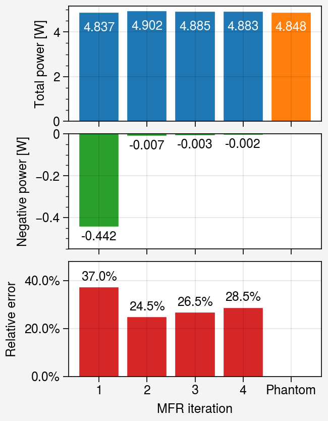
In this example, the minimum relative error is achieved at the 2nd iteration.
Solution basis history
Solution bases are also modified during the iteration and localized to the respective regions as the iteration progresses.
[21]:
for j, reg in enumerate(regs):
    fig, axes = uplt.subplots(ncols=6, refwidth=1, wspace=0.0)

    for i, ax in enumerate(axes):
        profile2d = np.full(voxel_map.shape, np.nan)
        profile2d[mask] = reg.basis[:, i]

        absolute = max(abs(svd.basis[:, i].min()), abs(svd.basis[:, i].max()))
        norm = AsinhNorm(vmin=-1 * absolute, vmax=absolute, linear_width=absolute * 1e-1)

        ax.imshow(
            profile2d.T,
            origin="lower",
            extent=(rmin, rmax, zmin, zmax),
            norm=norm,
        )

        ax.format(
            uctitle=f"basis {i}",
        )

    axes.format(
        ylabel=f"Iteration {j + 1}",
        ytickloc="neither",
        xtickloc="neither",
    )
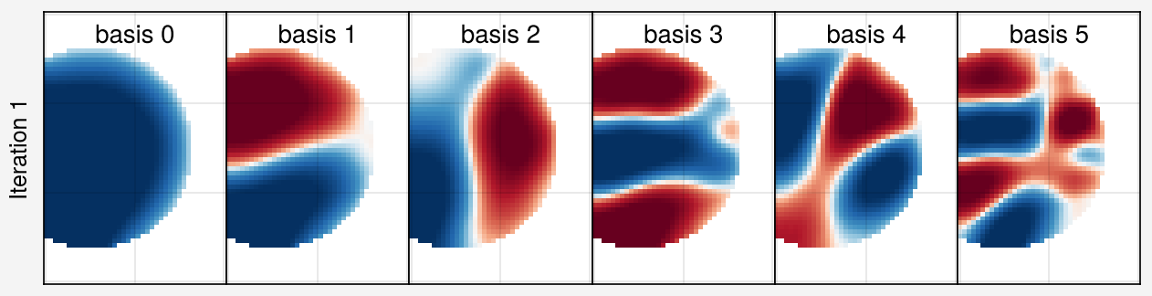

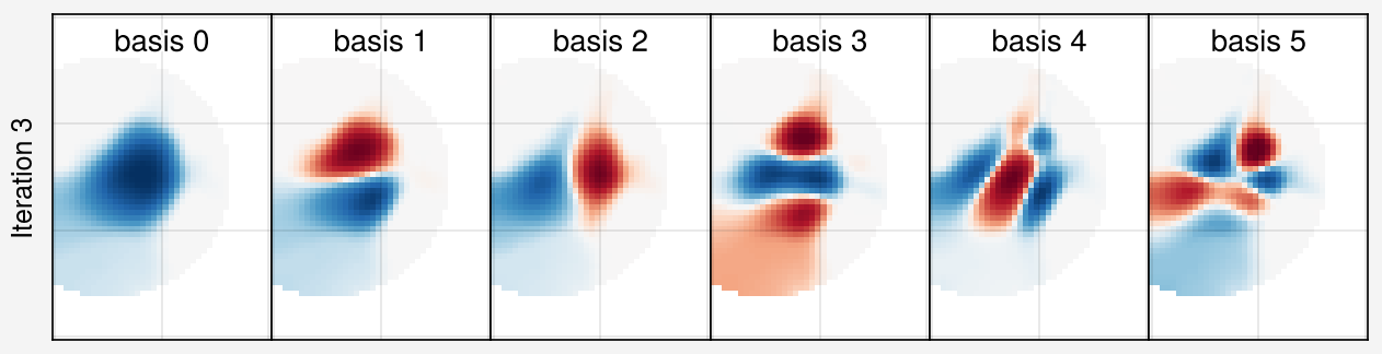
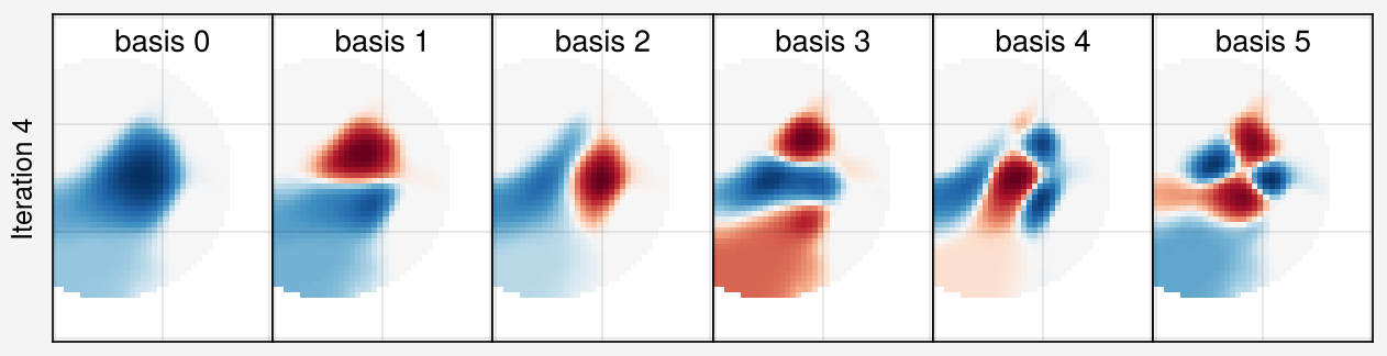
As the iteration progresses, the solution bases expand towards the left and bottom edges. This is likely due to the absence of boundary restrictions from backward difference derivatives.
To achieve a solution of zero at the boundary, anisotropic smoothing regularization is applied. This involves using numerical derivative matrices based on different coordinate systems, such as the polar coordinate system.
If you’d like to see an example of anisotropic smoothing regularization using derivative matrices derived from different schemes, check out the MFR tomography with anisotropic smoothing example.