Download notebook.
MFR tomography with anisotropic smoothing
On this page, we try to solve the same inversion problem as in the previous page, but with anisotropic smoothing. We will use the same dataset and model, but we will change the derivative matrix according to the gradient of the scalar function. Therefore, please compare the results of this page with the previous one to see the effect of the anisotropy.
[1]:
import pickle
from pathlib import Path
from pprint import pprint

import numpy as np
import ultraplot as uplt

from cherab.inversion import MFR, Lcurve
from cherab.inversion.data import get_sample_data
from cherab.inversion.tools import Derivative

# path to the directory to store the MFR results
store_dir = Path().cwd() / "02-mfr"
store_dir.mkdir(exist_ok=True)
Prepare the data
Load the same data as in the previous tomography example.
[2]:
# Load the sample data
grid_data = get_sample_data("bolo.npz")

# Extract the data
grids = grid_data["grid_centres"]
voxel_map = grid_data["voxel_map"].squeeze()
mask = grid_data["mask"].squeeze()
T = grid_data["sensitivity_matrix"]

print(f"{grids.shape = }")
print(f"{voxel_map.shape = }")
print(f"{mask.shape = }")
print(f"{T.shape = }")
print(f"T density: {np.count_nonzero(T) / T.size:.2%}")
grids.shape = (40, 60, 2)
voxel_map.shape = (40, 60)
mask.shape = (40, 60)
T.shape = (48, 1210)
T density: 8.35%
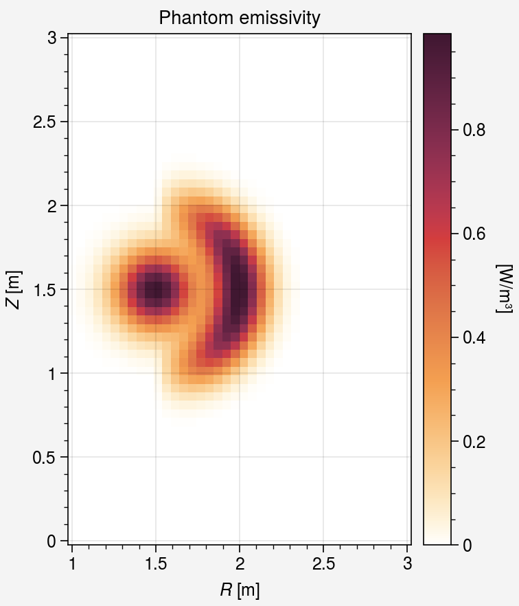
Define Phantom emission profile
The emission profile remains unchanged.
[3]:
PLASMA_AXIS = np.array([1.5, 1.5])
LCFS_RADIUS = 1
RING_RADIUS = 0.5

RADIATION_PEAK = 1
CENTRE_PEAK_WIDTH = 0.05
RING_WIDTH = 0.025


def emission_function_2d(rz_point: np.ndarray) -> float:
    direction = rz_point - PLASMA_AXIS
    bearing = np.arctan2(direction[1], direction[0])

    # calculate radius of coordinate from magnetic axis
    radius_from_axis = np.hypot(*direction)
    closest_ring_point = PLASMA_AXIS + (0.5 * direction / radius_from_axis)
    radius_from_ring = np.hypot(*(rz_point - closest_ring_point))

    # evaluate pedestal -> core function
    if radius_from_axis <= LCFS_RADIUS:
        central_radiatior = RADIATION_PEAK * np.exp(-(radius_from_axis**2) / CENTRE_PEAK_WIDTH)

        ring_radiator = (
            RADIATION_PEAK * np.cos(bearing) * np.exp(-(radius_from_ring**2) / RING_WIDTH)
        )
        ring_radiator = max(0, ring_radiator)

        return central_radiatior + ring_radiator
    else:
        return 0


# Create a 2-D phantom
nr, nz = voxel_map.shape
phantom_2d = np.full((nr, nz), np.nan)
for ir, iz in np.ndindex(nr, nz):
    if not mask[ir, iz]:
        continue
    phantom_2d[ir, iz] = emission_function_2d(grids[ir, iz])

# Create a 1-D phantom for the inversion
phantom = phantom_2d[mask]
[4]:
fig, ax = uplt.subplots()
image = ax.pcolormesh(
    grids[:, 0, 0],
    grids[0, :, 1],
    phantom_2d.T,
    discrete=False,
    colorbar="r",
    colorbar_kw=dict(label="[W/m³]", pad=0.0),
)
ax.format(
    aspect="equal",
    xlabel="$R$ [m]",
    ylabel="$Z$ [m]",
    title="Phantom emissivity",
)
Compute the measurement data
Let us prepare the measurement data \(\mathbf{b}\) using the geometry matrix \(\mathbf{T}\): \(\mathbf{b} = \mathbf{T} \mathbf{x} + \mathbf{e}\), where \(\mathbf{e}\) represents the noise. We will introduce 10% Gaussian noise based on the maximum value of the measurement data.
[5]:
T /= 4.0 * np.pi  # Divide by 4π steradians for use with power measurements in [W]
data = T @ phantom

rng = np.random.default_rng()
data_w_noise = data + rng.normal(0, data.max() * 1.0e-2, data.size)
data_w_noise = np.clip(data_w_noise, 0, None)
Anisotropic smoothing matrix \(\mathbf{H}\)
Definition
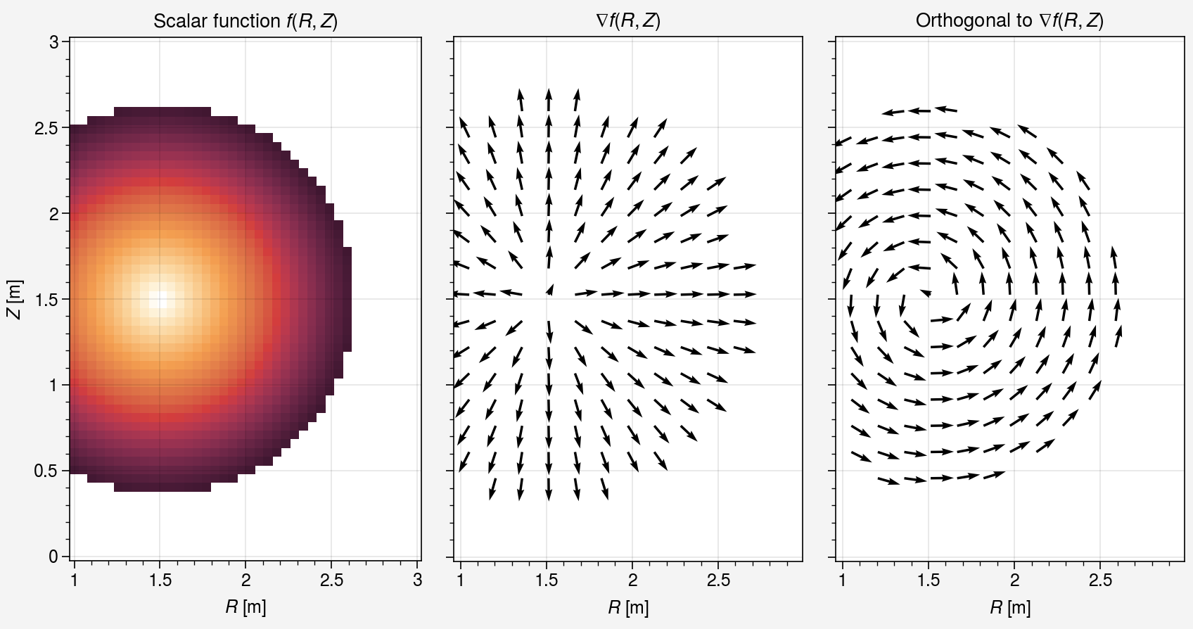
To apply the anisotropic smoothing, we propose the following anisotropic smoothing matrix (regularization matrix) \(\mathbf{H}\) [1] :
where \(\mathbf{D}_\parallel\) and \(\mathbf{D}_\perp\) are derivative matrices in the parallel directions along the gradient of a specific scalar function, \(\nabla f(R, Z)\), and perpendicular to it, respectively. The degree of anisotropy is determined by the coefficient \(\mathrm{sig}(\alpha)\), which is the sigmoid function with a parameter \(\alpha\) that regulates the strength of the anisotropy.
The differentiation of \(\mathbf{D}_\parallel\) and \(\mathbf{D}_\perp\) depends on the scalar function \(f(R, Z)\). We utilize a simple monotonically increasing function from the point \((R_0, Z_0)\), defined as follows:
The gradient and its orthogonal vector are shown below.
[6]:
def scalar_func(r, z):
    """Scalar function to be used for the demonstration."""
    return np.hypot(r - PLASMA_AXIS[0], z - PLASMA_AXIS[1])


# Compute scalar function values at each grid point.
fvals = np.zeros_like(grids[:, :, 0])
for ir, iz in np.ndindex(grids.shape[:2]):
    fvals[ir, iz] = scalar_func(grids[ir, iz, 0], grids[ir, iz, 1])

# Compute gradients of scalar function
grad_r, grad_z = np.gradient(fvals, grids[:, 0, 0], grids[0, :, 1])

# Mask values outside the plasma
fvals[voxel_map < 0] = np.nan
grad_r[voxel_map < 0] = np.nan
grad_z[voxel_map < 0] = np.nan

# Let us show the scalar function, its gradient, and orthogonal vectors.
fig, axes = uplt.subplots(ncols=3, spanx=False)
ax1, ax2, ax3 = axes

ax1.pcolormesh(
    grids[:, 0, 0],
    grids[0, :, 1],
    fvals.T,
    discrete=False,
)
ax1.format(
    aspect="equal",
    title="Scalar function $f(R, Z)$",
)

ax2.quiver(
    grids[:, 0, 0][1::3],
    grids[0, :, 1][::3],
    grad_r[1::3, ::3].T,
    grad_z[1::3, ::3].T,
    scale=15,
    color="black",
    width=0.007,
)
ax2.format(
    aspect="equal",
    title="$\\nabla f(R,Z)$",
)

ax3.quiver(
    grids[:, 0, 0][1::3],
    grids[0, :, 1][::3],
    -grad_z[1::3, ::3].T,
    grad_r[1::3, ::3].T,
    scale=15,
    color="black",
    width=0.007,
)
ax3.format(
    aspect="equal",
    title="Orthogonal to $\\nabla f(R,Z)$",
)

axes.format(
    xlabel="$R$ [m]",
    ylabel="$Z$ [m]",
)
Derivative matrices can be generated with the matrix_gradient method in the Derivative class.
[7]:
deriv = Derivative(grids, voxel_map)
dmat_para, dmat_perp = deriv.matrix_gradient(scalar_func)

dmat_pairs = [(dmat_para, dmat_para), (dmat_perp, dmat_perp)]
pprint(dmat_pairs)
[(<Compressed Sparse Row sparse array of dtype 'float64'
        with 3557 stored elements and shape (1210, 1210)>,
  <Compressed Sparse Row sparse array of dtype 'float64'
        with 3557 stored elements and shape (1210, 1210)>),
 (<Compressed Sparse Row sparse array of dtype 'float64'
        with 3609 stored elements and shape (1210, 1210)>,
  <Compressed Sparse Row sparse array of dtype 'float64'
        with 3609 stored elements and shape (1210, 1210)>)]
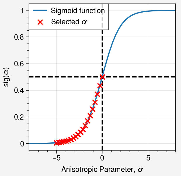
Optimize the anisotropic parameter \(\alpha\)
When reconstructing the profile, we need to choose the optimal value of the anisotropic parameter \(\alpha\), which is often optimized by reconstructing several test cases and seeking the best solution in terms of some criteria (e.g. relative error, SSIM, RMSD, etc.).
Because the phantom profile in this example is spread out in the circumferential direction to some extent, we try to strengthen the anisotropy in the same direction: set the anisotropic parameter \(\alpha\) to be negative. Let us plot the sigmoid function with setting parameters \(\alpha\).
[8]:
def sigmoid(x):
    """Sigmoid function."""
    return 1 / (1 + np.exp(-x))
[9]:
x = np.linspace(-8, 8)
alphas = np.linspace(-5, 0, 20)  # selected alphas

fig, ax = uplt.subplots()
ax.plot(x, sigmoid(x), label="Sigmoid function", zorder=0)
ax.scatter(alphas, sigmoid(alphas), marker="x", color="red", label="Selected $\\alpha$")
ax.axhline(0.5, color="black", linestyle="--", zorder=-1)
ax.axvline(0, color="black", linestyle="--", zorder=-1)
ax.legend(ncols=1)
ax.format(
    xlabel="Anisotropic Parameter, $\\alpha$",
    ylabel="$\\mathrm{sig}(\\alpha)$",
)
Let us define criterion functions: relative error \(\varepsilon_\mathrm{rel}\) and structural similarity index \(\mathrm{SSIM}\). They are given as follows:
where \(\mathbf{x}_\mathrm{true}\) is the true profile, \(\mathbf{x}_\mathrm{rec}\) is the reconstructed profile, \(\mu_x, \mu_y\) are the average values of \(\mathbf{x}_\mathrm{true}\) and \(\mathbf{x}_\mathrm{rec}\), respectively, \(\sigma_x, \sigma_y\) are the standard deviations of \(\mathbf{x}_\mathrm{true}\) and \(\mathbf{x}_\mathrm{rec}\), respectively, \(\sigma_{xy}\) is the covariance of \(\mathbf{x}_\mathrm{true}\) and \(\mathbf{x}_\mathrm{rec}\), \(C_1, C_2\) are constants, and \(\|\cdot\|\) is the Euclidean norm. Here \(C_1 = (k_1L)^2, C_2 = (k_2L)^2\) are constants, where \(k_1=0.01, k_2=0.03\), and \(L\) is the dynamic range of the profile values.
[10]:
def relative_error(x, true):
    """Compute relative error."""
    return np.linalg.norm(true - x) / np.linalg.norm(true)


def ssim(x, y):
    """Compute Structural Similarity Index."""
    ux, uy = np.mean(x), np.mean(y)
    vx, vy = np.var(x), np.var(y)
    vxy = (x - ux) @ (y - uy) / (x.size - 1)
    x_range, y_range = x.max() - x.min(), y.max() - y.min()
    data_range = max(x_range, y_range)
    c1, c2 = (0.01 * data_range) ** 2, (0.03 * data_range) ** 2
    return (2 * ux * uy + c1) * (2 * vxy + c2) / ((ux**2 + uy**2 + c1) * (vx + vy + c2))
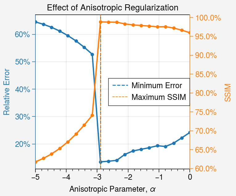
Let us try to solve the problem with the MFR method varying the anisotropic parameter \(\alpha\).
[11]:
num_mfi = 4  # number of MFR iterations
eps = 1.0e-6  # small positive number to avoid division by zero
tol = 1.0e-2  # tolerance for the convergence criterion

mfr = MFR(T, dmat_pairs, data=data_w_noise)

errors = []
ssims = []

for alpha in alphas:
    sol, stats = mfr.solve(
        derivative_weights=[sigmoid(alpha), sigmoid(-alpha)],
        miter=num_mfi,
        eps=eps,
        tol=tol,
        store_regularizers=False,
        spinner=False,
    )
    errors.append(relative_error(sol, phantom))
    ssims.append(ssim(phantom, sol))
Plot the relative error and SSIM for each \(\alpha\). Lower relative error and higher SSIM are better.
[12]:
fig, ax1 = uplt.subplots()
ax2 = ax1.alty(color="C1")

# Plot the relative error
ax1.plot(alphas, errors, marker=".")
line1 = ax1.axvline(
    alphas[np.argmin(errors)],
    color="C0",
    linestyle="--",
    lw=1,
    label="Minimum Error",
)
ax1.format(
    ycolor="C0",
    xlabel="Anisotropic Parameter, $\\alpha$",
    ylabel="Relative Error",
    title="Effect of Anisotropic Regularization",
    yformatter=("percent", 1),
)

# Plot the SSIM
ax2.plot(alphas, ssims, marker=".", color="C1")
line2 = ax2.axvline(
    alphas[np.argmax(ssims)],
    color="C1",
    linestyle="--",
    lw=0.7,
    label="Maximum SSIM",
)

lines = [line1, line2]
ax2.legend(
    lines,
    [line.get_label() for line in lines],
    ncols=1,
)

ax2.format(
    ylabel="SSIM",
    yformatter=("percent", 1),
)
Evaluate the best reconstruction with the optimized \(\alpha\)
We are assessing the optimal reconstruction using the optimized parameter \(\alpha\), which aims to maximize the SSIM.
[13]:
opt_alpha = alphas[np.argmax(ssims)]

sol, stats = mfr.solve(
    derivative_weights=[sigmoid(opt_alpha), sigmoid(-opt_alpha)],
    miter=num_mfi,
    eps=eps,
    tol=tol,
    store_regularizers=True,
    spinner=False,
    path=store_dir,
)
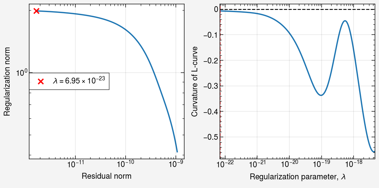
Let’s plot the L-curve and its curvature to use as a regularization criterion, so we can determine the optimal value of the regularization parameter.
[14]:
svd = stats["regularizer"]
fig, axes = uplt.subplots(ncols=2, share=False)
lcurve = Lcurve()
lcurve.plot_L_curve(svd, axes=axes[0])
lcurve.plot_curvature(svd, axes=axes[1])
axes[0].format(
    yformatter="log",
)
axes.format(
    xformatter="log",
)
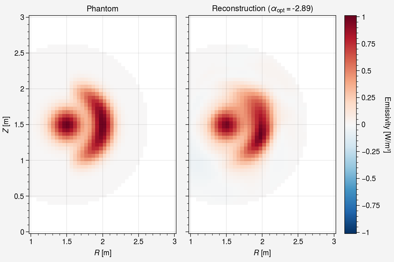
Compare profiles
Now, we will compare the reconstructed profile with the phantom and assess the quality of the reconstruction.
[15]:
vmax = max(np.abs(phantom).max(), np.abs(sol).max())

fig, axes = uplt.subplots(ncols=2, spanx=False)
for ax, profile, label in zip(
    axes,
    [phantom, sol],
    ["Phantom", f"Reconstruction ($\\alpha_{{\\mathrm{{opt}}}} = ${opt_alpha:.2f})"],
    strict=True,
):
    profile_2d = np.full(voxel_map.shape, np.nan)
    profile_2d[mask] = profile

    mappable = ax.pcolormesh(
        grids[:, 0, 0],
        grids[0, :, 1],
        profile_2d.T,
        discrete=False,
        vmin=-vmax,
        vmax=vmax,
    )
    ax.format(title=label)

fig.colorbar(
    mappable,
    ax=axes,
    label="Emissivity [W/m³]",
)

axes.format(
    aspect="equal",
    xlabel="$R$ [m]",
    ylabel="$Z$ [m]",
)
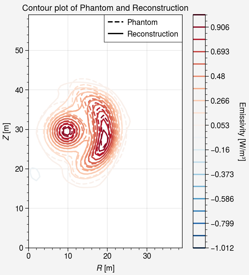
[16]:
dr, dz = grids[1, 0, 0] - grids[0, 0, 0], grids[0, 1, 1] - grids[0, 0, 1]
rmin, rmax = grids[0, 0, 0] - dr * 0.5, grids[-1, 0, 0] + dr * 0.5
zmin, zmax = grids[0, 0, 1] - dz * 0.5, grids[0, -1, 1] + dz * 0.5

vmax = max(np.amax(np.abs(sol)), np.amax(np.abs(phantom)))
levels = np.linspace(-vmax, vmax, 20)
sol_2d = np.full_like(phantom_2d, np.nan)
sol_2d[mask] = sol

fig, ax = uplt.subplots()
for profile, ls in zip([phantom_2d, sol_2d], ["--", "-"], strict=True):
    mappable = ax.contour(
        profile.T,
        vmin=-vmax,
        vmax=vmax,
        linestyles=ls,
        levels=levels,
        extent=[rmin, rmax, zmin, zmax],
    )

ax.colorbar(
    mappable,
    label="Emissivity [W/m³]",
)

ax.catlegend(
    ["Phantom", "Reconstruction"],
    line={"Phantom": True, "Reconstruction": True},
    linestyle={"Phantom": "--", "Reconstruction": "-"},
    linewidth={"Phantom": 1.5, "Reconstruction": 1.5},
    markers={"Phantom": "", "Reconstruction": ""},
    colors={"Phantom": "k", "Reconstruction": "k"},
    loc="upper right",
    ncols=1,
)

ax.format(
    aspect="equal",
    xlabel="$R$ [m]",
    ylabel="$Z$ [m]",
    title="Contour plot of Phantom and Reconstruction",
)
Compare the measurement powers
The measured power calculated by multiplying the geometry matrix by the emission vector and the back-calculated power calculated by multiplying the geometry matrix by the inverted emissivity are all in good agreement.
[17]:
back_calculated_measurements = T @ sol

fig, axes = uplt.subplots(
    nrows=2,
    refaspect=2.2,
    refwidth=5,
    sharey=False,
)
ax1, ax2 = axes

# Plot the phantom and the back-calculated measurements
ax1.bar(np.arange(data.size), data, label="Matrix-based measurements")
ax1.plot(back_calculated_measurements, ".", color="C1", label="Back-calculated from inversion")
ax1.legend(ncols=1)
ax1.format(
    ylabel="Power [W]",
)

# Plot the residuals between the measurements b and the back-calculated Tx (b - Tx)
ax2.axhline(0, color="k", linestyle="--")
ax2.bar(np.arange(data.size), data - back_calculated_measurements, color="C2")
ax2.format(
    ylabel="Residual [W]",
)

axes.format(
    xlim=(-1, data.size),
    xlabel="channel of bolometers",
    xlocator=5,
    xminorlocator=1,
)
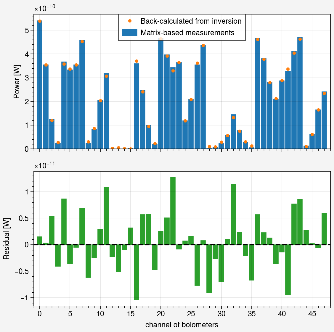
[18]:
print(
    "The relative error of power measurements is",
    f"{relative_error(back_calculated_measurements, data):.2%}",
)
The relative error of power measurements is 2.05%
Quantitative evaluation
We evaluate the reconstruction quality by measuring quantitative metrics such as relative error, SSIM, and the total/negative power of the reconstructed profile.
[19]:
dr = grids[1, 0, 0] - grids[0, 0, 0]
dz = grids[0, 1, 1] - grids[0, 0, 1]

volumes = dr * dz * 2.0 * np.pi * grids[..., 0]
volumes = volumes[mask]

print(f"Relative error : {relative_error(sol, phantom):.2%}")
print(f"SSIM           : {ssim(sol, phantom):.2%}")
print("--------------------------------------------")
print(f"Total power of phantom       : {phantom @ volumes:.4g} W")
print(f"Total power of reconstruction: {sol @ volumes:.4g} W")
print(f"Total negative power of reconstruction: {sol[sol < 0] @ volumes[sol < 0]:.4g} W")
Relative error : 13.45%
SSIM           : 98.85%
--------------------------------------------
Total power of phantom       : 4.848 W
Total power of reconstruction: 4.865 W
Total negative power of reconstruction: -0.08132 W
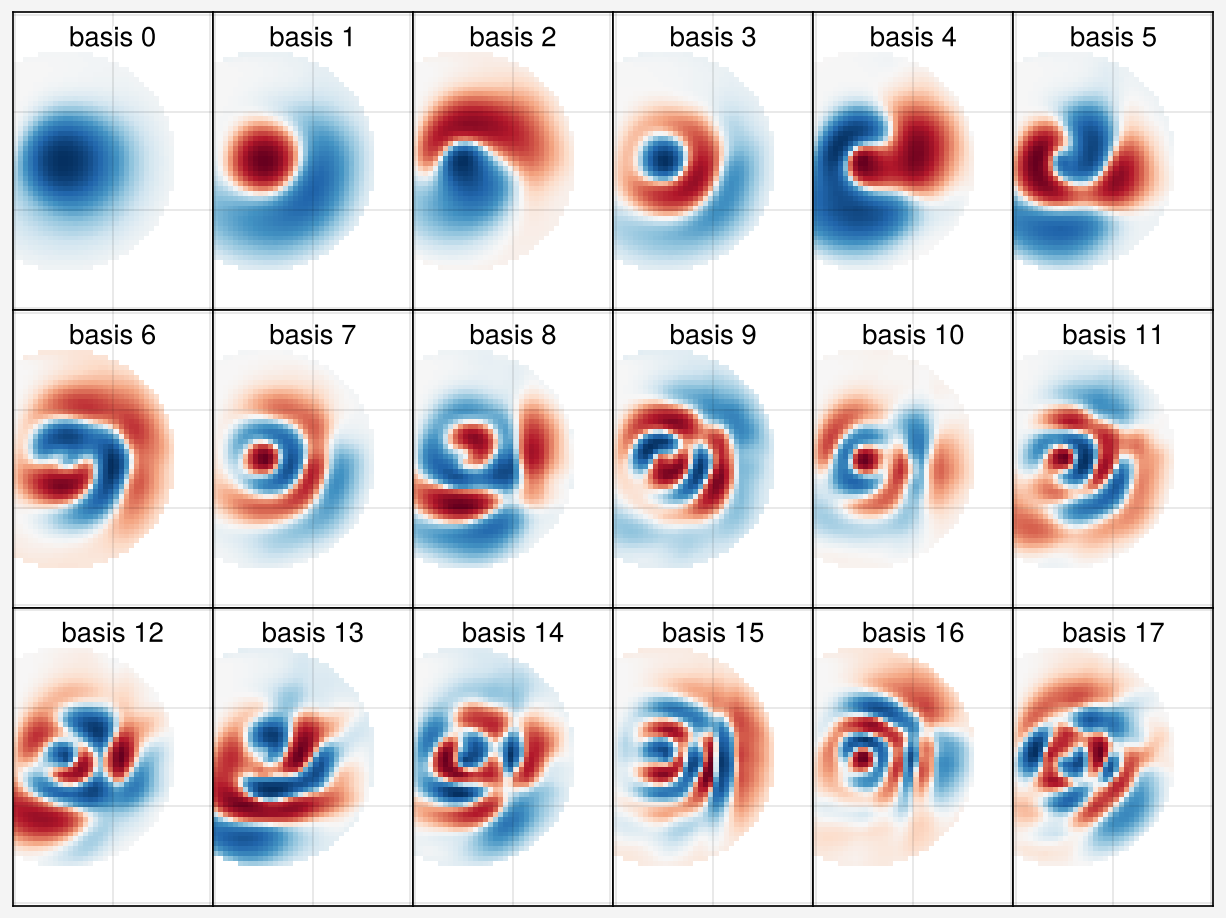
Solution basis
The solution bases from 0-th to 18-th are shown below.
[20]:
from matplotlib.colors import AsinhNorm

fig, axes = uplt.subplots(nrows=3, ncols=6, space=0.0, refwidth=1)

for i, ax in enumerate(axes):
    profile2d = np.full(voxel_map.shape, np.nan)
    profile2d[mask] = svd.basis[:, i]

    absolute = max(abs(svd.basis[:, i].min()), abs(svd.basis[:, i].max()))

    ax.imshow(
        profile2d.T,
        origin="lower",
        extent=(rmin, rmax, zmin, zmax),
        norm=AsinhNorm(vmin=-1 * absolute, vmax=absolute, linear_width=absolute * 1e-1),
    )

    ax.format(
        uctitle=f"basis {i}",
    )

axes.format(
    xtickloc="neither",
    ytickloc="neither",
)
Iteration history
As described in the MFR definition section, MFR is the iterative method. To see the convergence behavior, we investigate the iteration history.
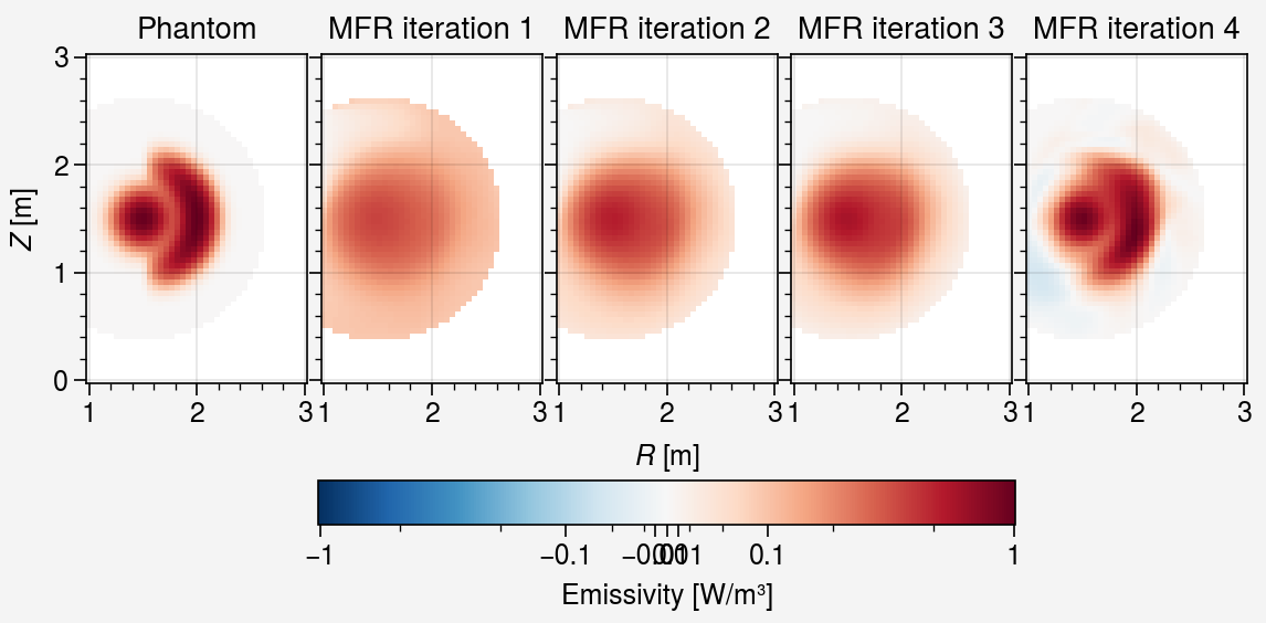
Reconstruction profiles history
Firstly, let’s examine the solution for each iteration. To address negative values, we will plot solutions using the arcsinh scale.
[21]:
# Stored regularizer files
reg_files = list(store_dir.glob("regularizer_*.pickle"))
reg_files = sorted(reg_files, key=lambda x: int(x.stem.split("_")[-1]))

# Load each solution
sols = []
regs = []
for file in reg_files:
    with open(file, "rb") as f:
        reg = pickle.load(f)

    sols.append(reg.solution(reg.lambda_opt))
    regs.append(reg)

profiles = [phantom] + sols

# set vmin and vmax for all solutions
vmin = min(profile.min() for profile in profiles)
vmax = max(profile.max() for profile in profiles)


# Plot the solutions
fig, axes = uplt.subplots(ncols=len(profiles), wspace=0.5, refwidth=1)

absolute = max(abs(vmax), abs(vmin))
linear_width = absolute * 0.1
norm = AsinhNorm(linear_width=linear_width, vmin=-1 * absolute, vmax=absolute)
i = 0
for ax, profile in zip(axes, profiles, strict=True):
    sol_2d = np.full(voxel_map.shape, np.nan)
    sol_2d[mask] = profile

    im = ax.imshow(
        sol_2d.T,
        origin="lower",
        extent=(rmin, rmax, zmin, zmax),
        norm=norm,
    )
    if i == 0:
        ax.format(title="Phantom")
    else:
        ax.format(title=f"MFR iteration {i}")
    i += 1

fig.colorbar(
    im,
    ax=axes,
    loc="b",
    shrink=0.6,
    label="Emissivity [W/m³]",
)

axes.format(
    xlabel="$R$ [m]",
    ylabel="$Z$ [m]",
)
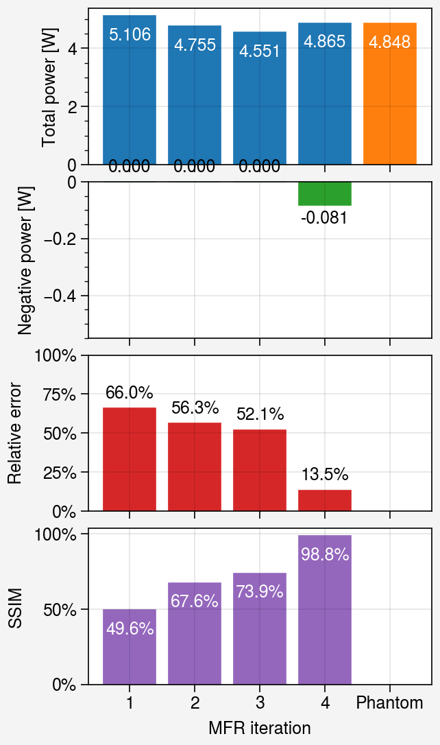
Quantitative evaluation history
The following plots show the quantitative evaluation changes during the iteration.
[22]:
relative_errors = []
total_powers = []
negative_powers = []
ssims = []

for sol in sols:
    relative_errors.append(relative_error(sol, phantom))
    total_powers.append(sol @ volumes)
    negative_powers.append(sol[sol < 0] @ volumes[sol < 0])
    ssims.append(ssim(phantom, sol))

# Append nan value to the last iteration
relative_errors.append(np.nan)
negative_powers.append(np.nan)
ssims.append(np.nan)

# show each value as a bar plot
fig, axes = uplt.subplots(nrows=4, sharey=False, refaspect=2.2, hspace=1)
ax1, ax2, ax3, ax4 = axes

x = np.arange(1, len(relative_errors) + 1)  # the label locations
rects = ax1.bar(
    x,
    total_powers + [np.sum(phantom * volumes)],
    color=["C0"] * (len(total_powers)) + ["C1"],
)
ax1.bar_label(rects, padding=-15, fmt="{:.3f}", color="w")
ax1.format(ylabel="Total power [W]")


rects = ax2.bar(x, negative_powers, color="C2")
ax2.bar_label(rects, padding=3, fmt="{:.3f}")
ax2.format(
    ylim=(-0.55, None),
    ylabel="Negative power [W]",
)

rects = ax3.bar(x, relative_errors, color="C3")
ax3.bar_label(rects, padding=3, fmt="{:.1%}")
ax3.format(
    ylim=(None, 1),
    ylabel="Relative error",
    yformatter=("percent", 1),
)

reacts4 = ax4.bar(x, ssims, color="C4")
ax4.bar_label(reacts4, padding=-15, fmt="{:.1%}", color="w")
ax4.format(
    ylabel="SSIM",
    yformatter=("percent", 1),
)

xlabels = [f"{s}" for s in x.tolist()[:4]] + ["Phantom"]
axes.format(
    xlabel="MFR iteration",
    xlocator=x,
    xticklabels=xlabels,
)
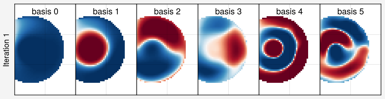
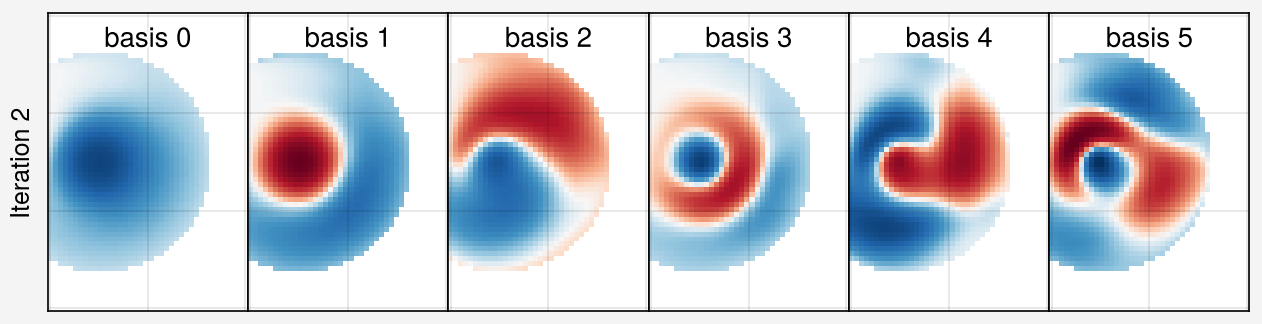
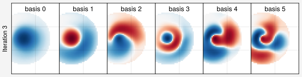
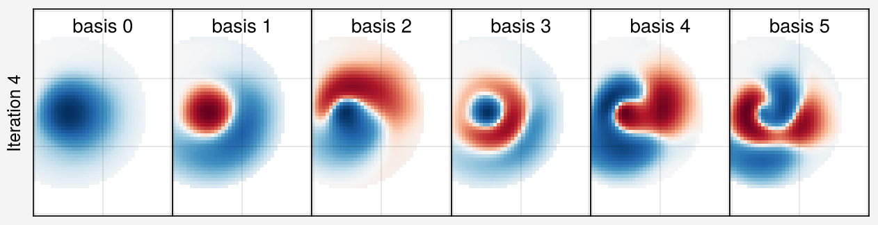
Solution basis history
Solution bases are altered and localized to specific regions during the iteration process.
[23]:
for j, reg in enumerate(regs):
    fig, axes = uplt.subplots(ncols=6, refwidth=1, wspace=0.0)

    for i, ax in enumerate(axes):
        profile2d = np.full(voxel_map.shape, np.nan)
        profile2d[mask] = reg.basis[:, i]

        absolute = max(abs(svd.basis[:, i].min()), abs(svd.basis[:, i].max()))
        norm = AsinhNorm(vmin=-1 * absolute, vmax=absolute, linear_width=absolute * 1e-1)

        ax.imshow(
            profile2d.T,
            origin="lower",
            extent=(rmin, rmax, zmin, zmax),
            norm=norm,
        )

        ax.format(
            uctitle=f"basis {i}",
        )

    axes.format(
        ylabel=f"Iteration {j + 1}",
        ytickloc="neither",
        xtickloc="neither",
    )