Download notebook.
Compare criteria for regularization parameter selection
This notebook is aimed at analyzing the behavior of different regularization methods for discrete ill-posed problems with different types of noise. The referenced paper is [1].
[1]:
import numpy as np
import ultraplot as uplt
from rich import print as rprint
from rich.table import Table
from scipy.optimize import minimize_scalar
from scipy.sparse import diags_array

from cherab.inversion import SVD
from cherab.inversion.regularization.criteria import GCV, PRESS, Lcurve
from cherab.inversion.tools import parse_scientific_notation
[2]:
def relative_error(
    log_lambda: float,
    solver: SVD,
    x_t: np.ndarray | None = None,
    x_t_norm: float | None = None,
) -> float:
    """Calculate relative error."""
    beta = 10**log_lambda
    sol = solver.solution(beta=beta)
    if x_t is None or x_t_norm is None:
        raise ValueError("x_t and x_t_norm must be provided")
    return np.linalg.norm(x_t - sol, axis=0) / x_t_norm
Definition of the example problem
Let us consider the following kernel and solution function derived from the Fredholm integral equation of the first kind:
[3]:
def _func(s: float, t: float) -> float:
    return np.pi * (np.sin(s) + np.sin(t))


def kernel(s: float, t: float) -> float:
    """The kernel function."""
    u = _func(s, t)
    if u == 0:
        return (np.cos(s) + np.cos(t)) ** 2.0
    else:
        return ((np.cos(s) + np.cos(t)) * np.sin(u) / u) ** 2.0


def solution(t: float) -> float:
    """The solution function."""
    return 2.0 * np.exp(-4.0 * (t - 0.5) ** 2.0) + np.exp(-4.0 * (t + 0.5) ** 2.0)
Discrete \(s\) and \(t\) in the range \(\displaystyle\left[-\frac{\pi}{2}, \frac{\pi}{2}\right]\) are used and the noise-free data \(\bar{\mathbf{b}}\) is given by \(\bar{\mathbf{b}} = \mathbf{K}\mathbf{x}\).
[4]:
s = np.linspace(-0.5 * np.pi, 0.5 * np.pi, num=64, endpoint=True)
t = np.linspace(-0.5 * np.pi, 0.5 * np.pi, num=64, endpoint=True)

# discretize kernel
k_mat = np.zeros((s.size, t.size))
k_mat = np.array([[kernel(i, j) for j in t] for i in s])

# trapezoidal rule
k_mat[:, 0] *= 0.5
k_mat[:, -1] *= 0.5
k_mat *= t[1] - t[0]

# discretize solution
x_t = np.array([solution(i) for i in t])

# noise-free data
b_bar = k_mat @ x_t

print(f"{k_mat.shape = }")
print(f"{x_t.shape = }")
print(f"condition number of K is {np.linalg.cond(k_mat):.4g}")
k_mat.shape = (64, 64)
x_t.shape = (64,)
condition number of K is 4.034e+18
1. White noise
First we consider the case of uncorrelated errors (white noise), i.e., the elements \(e_i\) of the perturbation \(\mathbf{e}\) are normally distributed with zero mean and standard deviation \(10^{-3}\). Hence the right-hand side \(\mathbf{b}\) of the perturbed problem is given by \(\mathbf{b} = \bar{\mathbf{b}} + \mathbf{e}\).
[5]:
rng = np.random.default_rng()
noise = rng.normal(0, 1.0e-3, b_bar.size)
b = b_bar + noise
The solution \(\mathbf{x}_\lambda = \left(\mathbf{K}^\mathsf{T}\mathbf{K} + \lambda\mathbf{I}\right)^{-1}\mathbf{K}^\mathsf{T}\mathbf{b}\) is computed and the regularization parameter \(\lambda\) is selected by several criteria.
[6]:
# SVD solver
svd = SVD(k_mat, data=b)

# Analyze different criteria
sols = {}
lambdas_opt = {}
errors = {}
x_t_norm = np.linalg.norm(x_t, axis=0)

for criterion in [PRESS(), GCV(), Lcurve()]:
    # Find optimal lambda and solution
    sol, _ = svd.solve(criterion)

    # Store results
    name = criterion.__class__.__name__
    sols[name] = sol
    lambdas_opt[name] = svd.lambda_opt
    errors[name] = relative_error(np.log10(svd.lambda_opt), svd, x_t, x_t_norm)
Get the minimum error solution by optimizing \(\lambda\) to minimize the relative error of the solution.
[7]:
res = minimize_scalar(
    relative_error,
    bounds=svd.bounds,
    method="bounded",
    args=(svd, x_t, x_t_norm),
    options={"xatol": 1.0e-10, "maxiter": 500},
)

# obtain minimum relative error and lambda
error_min = res.fun
lambda_min = 10**res.x
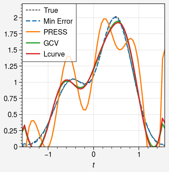
Show the results in a table and plot the optimal solutions for each criterion.
[8]:
table = Table(title="Comparison of different criteria")
table.add_column("Criterion", justify="center", style="cyan", no_wrap=True)
table.add_column("Optimal Lambda", justify="center", style="magenta")
table.add_column("Relative Error", justify="center", style="green")
for label in sols.keys():
    table.add_row(label, f"{lambdas_opt[label]:.2e}", f"{errors[label]:.2%}")

table.add_section()
table.add_row("Minimum Error", f"{lambda_min:.2e}", f"{error_min:.2%}")
rprint(table)
         Comparison of different criteria
┏━━━━━━━━━━━━━━━┳━━━━━━━━━━━━━━━━┳━━━━━━━━━━━━━━━━┓
┃   Criterion   ┃ Optimal Lambda ┃ Relative Error ┃
┡━━━━━━━━━━━━━━━╇━━━━━━━━━━━━━━━━╇━━━━━━━━━━━━━━━━┩
│     PRESS     │    1.54e-08    │     41.13%     │
│      GCV      │    7.49e-07    │     10.57%     │
│    Lcurve     │    3.36e-07    │     12.68%     │
├───────────────┼────────────────┼────────────────┤
│ Minimum Error │    4.88e-05    │     1.42%      │
└───────────────┴────────────────┴────────────────┘
[9]:
fig, ax = uplt.subplots()
ax.plot(t, x_t, ls="--", lw=0.75, color="k", label="True")
ax.plot(t, svd.solution(beta=lambda_min), ls="--", label="Min Error")
for label, sol in sols.items():
    ax.plot(t, sol, label=label)

ax.legend(ncols=1)
ax.format(
    ylim=(0, x_t.max() * 1.1),
    xlabel="$t$",
)
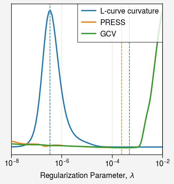
Plot each criterion as a function of \(\lambda\).
[10]:
fig, ax_origin = uplt.subplots()
lambdas = np.logspace(*svd.bounds, num=500)
hs = []
i = 0

# -------------------------
# === L-curve curvature ===
# -------------------------
lcurve = Lcurve()
(h,) = ax_origin.plot(
    lambdas,
    [lcurve.curvature(svd, beta=beta) for beta in lambdas],
    label="L-curve curvature",
)
ax_origin.axvline(lambdas_opt["Lcurve"], ls="--", color=f"C{i}", lw=0.75)
hs.append(h)
i += 1

# -------------
# === PRESS ===
# -------------
ax = ax_origin.alty()
press = PRESS()
(h,) = ax.plot(
    lambdas,
    [press.press(svd, beta=beta) for beta in lambdas],
    label="PRESS",
    color=f"C{i}",
)
ax.axvline(lambdas_opt["PRESS"], ls="--", color=f"C{i}", lw=0.75)
hs.append(h)
i += 1
ax.format(
    xscale="log",
    yscale="log",
    xformatter="log",
    ytickloc="none",
)

# -----------
# === GCV ===
# -----------
ax = ax_origin.alty()
gcv = GCV()
(h,) = ax.plot(
    lambdas,
    [gcv.gcv(svd, beta=beta) for beta in lambdas],
    label="GCV",
    color=f"C{i}",
)
ax.axvline(lambdas_opt["GCV"], ls="--", color=f"C{i}", lw=0.75)
hs.append(h)
i += 1
ax.format(
    xscale="log",
    yscale="log",
    xformatter="log",
    ytickloc="none",
)


# Legend
fig.legend(
    hs,
    ncols=1,
    ref=ax,
    loc="upper right",
)

# Final formatting
fig.format(
    xscale="log",
    xformatter="log",
    xlabel="Regularization Parameter, $\\lambda$",
    ytickloc="none",
    ygrid=False,
    xlim=(1e-8, 1e-2),
)
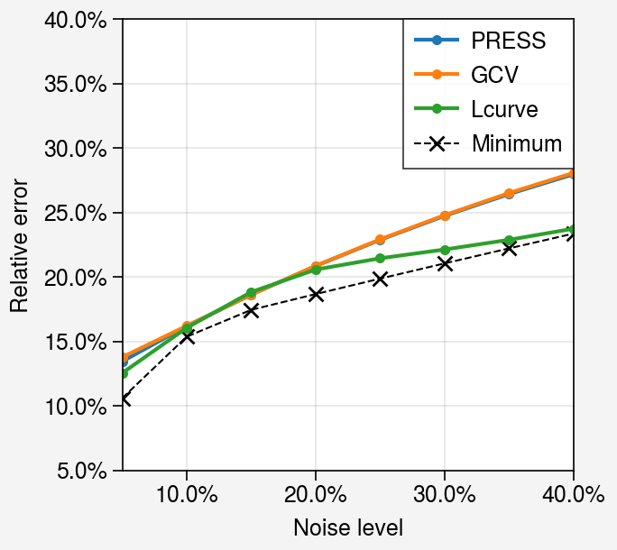
Behavior of different noise levels
Let us analyze the behavior of the criteria for different noise levels. We add different levels of white noise, from 5% to 40%, then plot the relative error of the optimal solutions for each criterion as a function of the noise level.
[11]:
noise_levels = np.arange(0.05, 0.45, 0.05)  # 5% to 40%
criteria_classes = [PRESS, GCV, Lcurve]

error_vs_noise = {cls.__name__: [] for cls in criteria_classes}
errors_min = []

e_origin = rng.normal(0.0, 1.0, size=b_bar.size)
e_origin_norm = np.linalg.norm(e_origin)

for level in noise_levels:
    # create white noise with prescribed relative level ||e|| / ||b_bar|| = level
    e = e_origin * (level * np.linalg.norm(b_bar)) / e_origin_norm
    b_noisy = b_bar + e

    svd_level = SVD(k_mat, data=b_noisy)

    for cls in criteria_classes:
        criterion = cls()
        sol, _ = svd_level.solve(criterion)
        err = float(np.linalg.norm(x_t - sol) / x_t_norm)
        error_vs_noise[cls.__name__].append(err)

    # Compute the minimum error for this noise level
    res = minimize_scalar(
        relative_error,
        bounds=svd_level.bounds,
        method="bounded",
        args=(svd_level, x_t, x_t_norm),
        options={"xatol": 1.0e-10, "maxiter": 500},
    )

    # obtain minimum relative error and lambda
    errors_min.append(res.fun)

fig, ax = uplt.subplots()
for name, errs in error_vs_noise.items():
    ax.plot(noise_levels, np.array(errs), marker=".", label=name)

ax.plot(
    noise_levels,
    np.array(errors_min),
    marker="x",
    ls="--",
    lw=0.75,
    color="k",
    label="Minimum",
    zorder=-1,
)

ax.legend(ncols=1)
ax.format(
    ylim=(noise_levels.min(), noise_levels.max()),
    xlabel="Noise level",
    ylabel="Relative error",
    xformatter=("percent", 1),
    yformatter=("percent", 1),
)
2. Uncorrelated noise
Next we consider the case of highly correlated errors, which are derived from a regular smoothing of the matrix \(\mathbf{K}\) and the right-hand side \(\bar{\mathbf{b}}\):
where \(\mu\) is set to \(0.05\) and the outside elements are set to zero.
[12]:
mu = 0.05

k_mat_smooth = np.zeros_like(k_mat)
b = np.zeros_like(b_bar)

for i in range(len(b_bar)):
    if i < 1:
        b[i] = b_bar[i] + mu * (0 + b_bar[i + 1])
    elif i > len(b_bar) - 2:
        b[i] = b_bar[i] + mu * (b_bar[i - 1] + 0)
    else:
        b[i] = b_bar[i] + mu * (b_bar[i - 1] + b_bar[i + 1])


for i, j in np.ndindex(*k_mat.shape):
    if i - 1 < 0:
        k1 = 0
    else:
        k1 = k_mat[i - 1, j]
    if i + 1 > k_mat.shape[0] - 1:
        k2 = 0
    else:
        k2 = k_mat[i + 1, j]
    if j - 1 < 0:
        k3 = 0
    else:
        k3 = k_mat[i, j - 1]
    if j + 1 > k_mat.shape[1] - 1:
        k4 = 0
    else:
        k4 = k_mat[i, j + 1]

    k_mat_smooth[i, j] = k_mat[i, j] + mu * (k1 + k2 + k3 + k4)
Show the results in a table.
[13]:
# SVD solver
svd = SVD(k_mat_smooth, data=b)

# Analyze different criteria
sols = {}
lambdas_opt = {}
errors = {}
x_t_norm = np.linalg.norm(x_t, axis=0)

for criterion in [PRESS(), GCV(), Lcurve()]:
    # Find optimal lambda and solution
    sol, _ = svd.solve(criterion)

    # Store results
    name = criterion.__class__.__name__
    sols[name] = sol
    lambdas_opt[name] = svd.lambda_opt
    errors[name] = relative_error(np.log10(svd.lambda_opt), svd, x_t, x_t_norm)
[14]:
# minimize relative error
res = minimize_scalar(
    relative_error,
    bounds=svd.bounds,
    method="bounded",
    args=(svd, x_t, x_t_norm),
    options={"xatol": 1.0e-10, "maxiter": 500},
)

# obtain minimum relative error and lambda
error_min = res.fun
lambda_min = 10**res.x
[15]:
table = Table(title="Comparison of different criteria")
table.add_column("Criterion", justify="center", style="cyan", no_wrap=True)
table.add_column("Optimal Lambda", justify="center", style="magenta")
table.add_column("Relative Error", justify="center", style="green")
for label in sols.keys():
    table.add_row(label, f"{lambdas_opt[label]:.2e}", f"{errors[label]:.2%}")

table.add_section()
table.add_row("Minimum Error", f"{lambda_min:.2e}", f"{error_min:.2%}")
rprint(table)
         Comparison of different criteria
┏━━━━━━━━━━━━━━━┳━━━━━━━━━━━━━━━━┳━━━━━━━━━━━━━━━━┓
┃   Criterion   ┃ Optimal Lambda ┃ Relative Error ┃
┡━━━━━━━━━━━━━━━╇━━━━━━━━━━━━━━━━╇━━━━━━━━━━━━━━━━┩
│     PRESS     │    8.17e-20    │   102836.57%   │
│      GCV      │    2.44e-27    │   396453.81%   │
│    Lcurve     │    1.73e-30    │   918829.09%   │
├───────────────┼────────────────┼────────────────┤
│ Minimum Error │    2.89e-05    │     8.49%      │
└───────────────┴────────────────┴────────────────┘
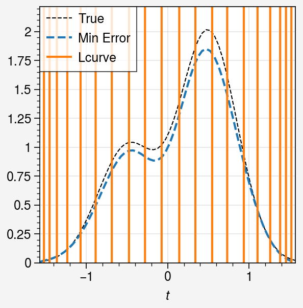
The L-curve method still works well, however, the other methods fail to find the optimal \(\lambda\).
Let us plot the optimal solutions as well as the original solution and the minimum-error one with only L-curve method.
[16]:
fig, ax = uplt.subplots()
ax.plot(t, x_t, ls="--", lw=0.75, color="k", label="True")
ax.plot(t, svd.solution(beta=lambda_min), ls="--", label="Min Error")
method = Lcurve.__name__
ax.plot(t, sols[method], label=method)

ax.legend(ncols=1)
ax.format(
    ylim=(0, x_t.max() * 1.1),
    xlabel="$t$",
)