GCV criterion
Here we show how to use the Generalized Cross Validation (GCV) criterion to select the optimal regularization parameter for an example ill-posed inverse problem.
The definition of the GCV criterion is introduced in this page.
Definition of the example problem
We refer to the famous Fredholm integral equation of the first kind devised by Phillips[1]. Define the function
Then, the kernel \(K(s, t)\) and the solution \(x(t)\) are given by
Both integral intervals are \([-6, 6]\).
[1]:
import numpy as np
import ultraplot as uplt
from rich import print as rprint
from scipy.sparse import diags_array

from cherab.inversion import GCV, SVD
from cherab.inversion.tools import parse_scientific_notation
Let us define functions for the kernel, the solution and the right-hand side.
[2]:
Then we will generate the discretized version of the kernel \(\mathbf{K}\), solution \(\mathbf{x}\) and right-hand side \(\mathbf{b}\) using the trapezoidal rule leading to the following linear system:
The size of matrix \(\mathbf{K}\in\mathbb{R}^{M\times N}\) is set to \(M = N = 64\).
[3]:
s = np.linspace(-6.0, 6.0, num=64, endpoint=True)
t = np.linspace(-6.0, 6.0, num=64, endpoint=True)

# discretize kernel
k_mat = np.zeros((s.size, t.size))
k_mat = np.array([[kernel(i, j) for j in t] for i in s])

# trapezoidal rule
k_mat[:, 0] *= 0.5
k_mat[:, -1] *= 0.5
k_mat *= t[1] - t[0]

# discretize solution
x_t = np.array([solution(i) for i in t])

print(f"{k_mat.shape = }")
print(f"{x_t.shape = }")
print(f"condition number of K is {np.linalg.cond(k_mat):.4g}")
k_mat.shape = (64, 64)
x_t.shape = (64,)
condition number of K is 5.924e+04
The right-hand side \(\mathbf{b}\in\mathbb{R}^{M}\) is usually contaminated by noise. So, we will add a Gaussian noise to the right-hand side.
where \(\bar{\mathbf{b}}\) is the original right-hand side (\(\bar{\mathbf{b}}\equiv \mathbf{K}\mathbf{x}\)), \(\mathbf{e}\) is a vector whose elements are independently sampled from the normal distribution with mean 0 and standard deviation \(10^{-3}\).
[4]:
b_bar = k_mat @ x_t
rng = np.random.default_rng()
noise = rng.normal(0, 1.0e-3, b_bar.size)
b = b_bar + noise
Solve the inverse problem using the GCV criterion
The solution of the ill-posed linear equation is obtained with the regularization procedure:
where \(\mathbf{H}\) is the regularization matrix. Here we set \(\mathbf{H} = \mathbf{D_2}^\mathsf{T}\mathbf{D_2}\), where \(\mathbf{D_2}\) is the second-order difference matrix.
[5]:
dmat = diags_array([1, -2, 1], offsets=[-1, 0, 1], shape=(t.size, t.size), dtype=float).tocsr()
print(f"{dmat.shape = }")
dmat.shape = (64, 64)
Then we create SVD solver object.
Let us solve the inverse problem with the GCV criterion to determine the optimal regularization parameter.
                    message: ['requested number of basinhopping iterations completed successfully']
                    success: True
                        fun: 1.5814610690558967e-08
                          x: [-2.103e+00]
                        nit: 100
      minimization_failures: 0
                       nfev: 534
                       njev: 267
 lowest_optimization_result:  message: CONVERGENCE: NORM OF PROJECTED GRADIENT <= PGTOL
                              success: True
                               status: 0
                                  fun: 1.5814610690558967e-08
                                    x: [-2.103e+00]
                                  nit: 0
                                  jac: [-2.517e-10]
                                 nfev: 2
                                 njev: 1
                             hess_inv: <1x1 LbfgsInvHessProduct with dtype=float64>
Evaluate the GCV criterion
Next we evaluate the solution obtained by the GCV criterion
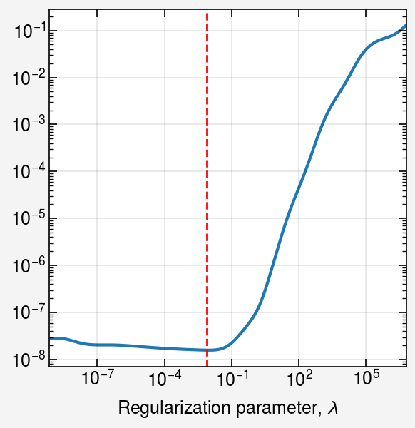
Plot GCV curve
[8]:
fig, ax = uplt.subplots()
gcv.plot_gcv(axes=ax)
ax.format(
    xformatter="log",
    yformatter="log",
)
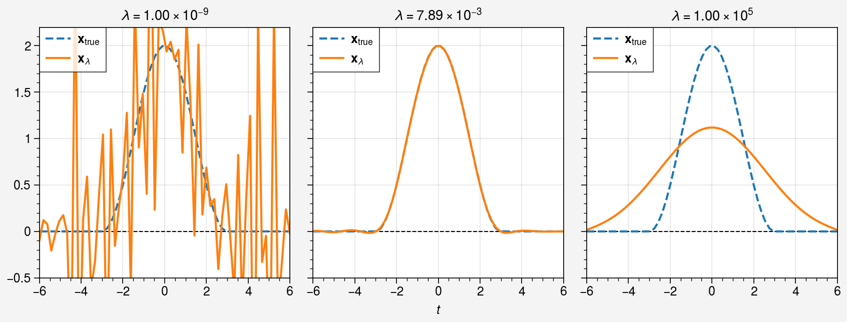
Compare \(\mathbf{x}_\lambda\) with \(\mathbf{x}_\mathrm{true}\)
Let us compare solutions at different regularization parameters \(\lambda=10^{-9}\), \(\lambda_\text{opt}\), \(10^5\) with the true solution \(\mathbf{x}_\mathrm{true}\).
[9]:
lambdas = [1.0e-9, svd.lambda_opt, 1.0e5]

fig, axes = uplt.subplots(ncols=3)

for ax, beta in zip(axes, lambdas, strict=False):
    ax.plot(t, x_t, "--", label="$\\mathbf{x}_\\mathrm{true}$")
    ax.plot(t, svd.solution(beta=beta), label="$\\mathbf{x}_\\lambda$")
    ax.axhline(0, color="black", lw=0.75, ls="--", zorder=-1)

    ax.legend(loc="upper left", ncols=1)

    parsed_lambda = parse_scientific_notation(f"{beta:.2e}")
    ax.format(
        title=f"$\\lambda = {parsed_lambda}$",
    )

axes.format(
    ylim=(-0.5, x_t.max() * 1.1),
    xlabel="$t$",
)
Check the relative error
The relative error between the solution \(\mathbf{x}_\lambda\) and the true solution \(\mathbf{x}_\mathrm{true}\) is defined as follows:
Let us seek the minimum \(\epsilon_\mathrm{rel}\) as a function of \(\lambda\).
[10]:
from scipy.optimize import minimize_scalar

X_T_NORM = np.linalg.norm(x_t, axis=0)


def relative_error(
    log_lambda: float,
    x_t: np.ndarray = x_t,
    x_t_norm: float = X_T_NORM,
    svd: SVD = svd,
) -> float:
    """Calculate relative error."""
    beta = 10**log_lambda
    sol = svd.solution(beta=beta)
    return np.linalg.norm(x_t - sol, axis=0) / x_t_norm


# minimize relative error
bounds = svd.bounds
res = minimize_scalar(
    relative_error,
    bounds=bounds,
    method="bounded",
    args=(x_t, X_T_NORM, svd),
    options={"xatol": 1.0e-10, "maxiter": 1000},
)

# obtain minimum relative error and lambda
error_min = res.fun
lambda_min = 10**res.x

print(f"minimum relative error: {error_min:.2%} at lambda = {lambda_min:.4g}")
minimum relative error: 0.73% at lambda = 0.008739
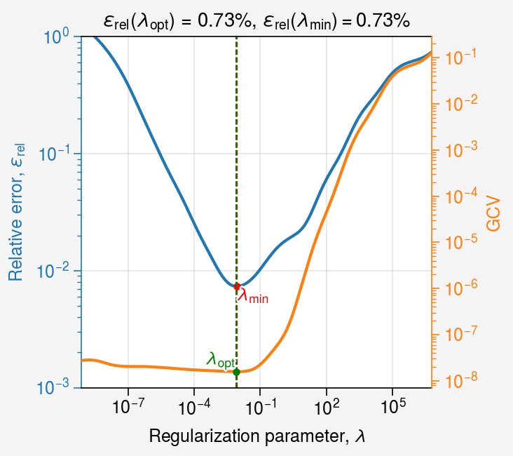
Let us plot the relative error and curvature as a function of \(\lambda\).
[11]:
# set regularization parameters
num = 500
lambdas = np.logspace(*bounds, num=num)

# calculate errors and gcv
errors = np.asarray([relative_error(log_lambda) for log_lambda in np.linspace(*bounds, num=num)])
gcvs = np.asarray([gcv.gcv(svd, beta) for beta in lambdas])

# create figure
fig, ax1 = uplt.subplots()
ax2 = ax1.alty(color="C1")

# plot errors and gcv
ax1.loglog(lambdas, errors, color="C0")
ax2.loglog(lambdas, gcvs, color="C1")

# plot minimum error vertical line and point
ax1.axvline(lambda_min, color="r", linestyle="--", linewidth=0.75)
ax1.scatter(lambda_min, error_min, color="r", marker="o", s=10, zorder=2)
ax1.text(
    lambda_min,
    error_min,
    "$\\lambda_\\mathrm{min}$",
    color="r",
    horizontalalignment="left",
    verticalalignment="top",
    border=True,
)

# plot minimum gcv vertical line and point
assert svd.lambda_opt is not None
min_gcv = gcv.gcv(svd, svd.lambda_opt)
ax1.axvline(svd.lambda_opt, color="g", linestyle="--", linewidth=0.75)
ax2.scatter(svd.lambda_opt, min_gcv, color="g", marker="o", s=10, zorder=2)
ax2.text(
    svd.lambda_opt,
    min_gcv,
    "$\\lambda_\\mathrm{opt}$",
    color="g",
    horizontalalignment="right",
    verticalalignment="bottom",
    border=True,
)

ax1.autoscale(enable=True, axis="x", tight=True)
ax2.autoscale(enable=True, axis="x", tight=True)

# format axes
ax1.format(
    ycolor="C0",
    ylim=(1.0e-3, 1),
    xlabel="Regularization parameter, $\\lambda$",
    ylabel="Relative error, $\\epsilon_\\mathrm{rel}$",
    xformatter="log",
    yformatter="log",
)
ax2.format(
    ylabel="GCV",
    yformatter="log",
)

error_opt = relative_error(np.log10(svd.lambda_opt))
ax1.format(
    title=f"$\\epsilon_\\mathrm{{rel}}(\\lambda_\\mathrm{{opt}})$ = {error_opt:.2%}, "
    + f"$\\epsilon_\\mathrm{{rel}}(\\lambda_\\mathrm{{min}}) = ${error_min:.2%}"
)