matrix_along_axis()

Derivative.matrix_along_axis(axis: int, diff_type: Literal['forward', 'backward'] = 'forward', boundary: Literal['dirichlet', 'neumann', 'periodic'] = 'dirichlet') → csr_arraySource

Derivative matrix along the specified axis.

Note

If the grid has masked area, edges before the masked area take either the dirichlet (forward) or neumann (backward) condition. The periodic boundary condition is only available for the last and first points along the axis.

Parameters:

axisint

The axis to calculate the derivative matrix. The axis must be in the grid dimensions.

diff_type{“forward”, “backward”}, optional

The type of the difference method, by default “forward”.

boundary{“dirichlet”, “neumann”, “periodic”}, optional

The boundary condition of the derivative matrix, by default “dirichlet”. If the boundary condition is “dirichlet”, the outer boundary is set to zero. If the boundary condition is “neumann”, the difference type is set to the opposite direction at the edge of the grid. If the boundary condition is “periodic”, the first and last points are connected.

Returns:

csr_array

The derivative matrix along the specified axis.

Examples

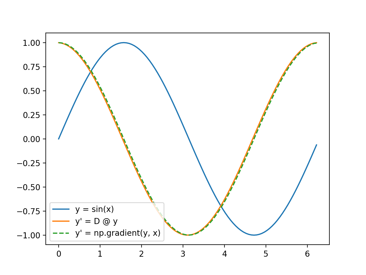
Firstly, let us operate the derivative matrix to a simple 1-D profile and compare it with gradient values calculated by the numpy.gradient function.

import numpy as np
import matplotlib.pyplot as plt
from cherab.inversion import Derivative

# Create a sample 1-D sine profile
x = np.linspace(0, 2 * np.pi, 100, endpoint=False)
y = np.sin(x)

# Calculate the derivative matrix
derivative = Derivative(x)
dmat = derivative.matrix_along_axis(0, boundary="dirichlet")

# Compare gradient values
plt.plot(x, y, label="y = sin(x)")
plt.plot(x, dmat @ y, label="y' = D @ y")
plt.plot(x, np.gradient(y, x), label="y' = np.gradient(y, x)", linestyle="--")
plt.legend()
plt.show()

(Source code, png, hires.png, pdf)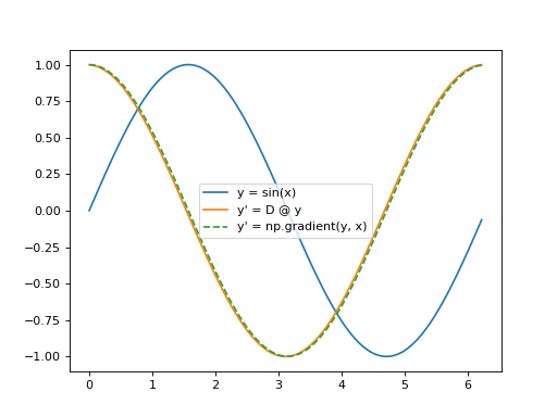

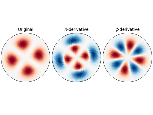
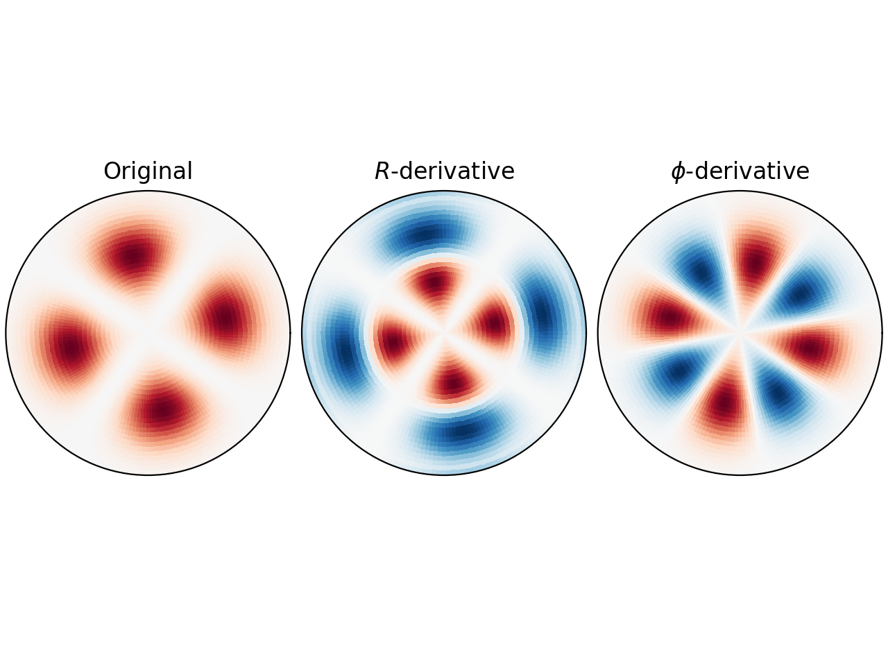
Next, we create a sample 2-D profile in cylindrical coordinates and apply the derivative along the R and Phi axis to the profile.

import numpy as np
from matplotlib import pyplot as plt
from matplotlib.gridspec import GridSpec

from cherab.inversion import Derivative

# R-Phi grids
radius = np.linspace(0.1, 1, 30)
angles = np.linspace(0, 2 * np.pi, 180, endpoint=False)

# Create voxels center coordinates in (x, y, z)
rr, pp = np.meshgrid(radius, angles)
centers = np.zeros((30, 180, 1, 3))
centers[:, :, 0, 0] = (rr * np.cos(pp)).T
centers[:, :, 0, 1] = (rr * np.sin(pp)).T
centers[:, :, 0, 2] = 0

# Create a 2-D profile
indices = np.ndindex(centers.shape[:3])
profile = np.zeros(centers.shape[:3])

CENTER = 0.6
WIDTH = 0.05
PHASE = -np.pi / 4
for ir, ip, iz in indices:
    profile[ir, ip, iz] = (1 + np.cos(angles[ip] * 4 + PHASE)) * np.exp(
        -((radius[ir] - CENTER) ** 2) / WIDTH
    )


# Operate derivative
deriv = Derivative(
    centers,
    np.arange(np.prod(centers.shape[:3]), dtype=np.int32).reshape(centers.shape[:3]),
)
dmat_r = deriv.matrix_along_axis(0, diff_type="forward", boundary="dirichlet")
dmat_p = deriv.matrix_along_axis(1, diff_type="forward", boundary="periodic")

profile_dr = dmat_r @ profile.ravel()
profile_dp = dmat_p @ profile.ravel()
profile_dr = profile_dr.reshape(centers.shape[:3])
profile_dp = profile_dp.reshape(centers.shape[:3])

# Plot the profiles
fig = plt.figure(layout="constrained")
gs = GridSpec(1, 3, figure=fig)
for i, (f, title) in enumerate(
    zip(
        [profile, profile_dr, profile_dp],
        ["Original", "$R$-derivative", "$\\phi$-derivative"],
        strict=True,
    )
):
    ax = fig.add_subplot(gs[i], projection="polar")
    ax.grid(False)
    ax.pcolormesh(
        angles,
        radius,
        f[..., 0],
        cmap="RdBu_r",
        vmax=np.amax(np.abs(f)),
        vmin=-np.amax(np.abs(f)),
    )
    ax.set_rticks([])
    ax.set_thetagrids([])
    ax.set_title(title)

plt.show()

(Source code, png, hires.png, pdf)