Note

This page was generated from notebooks/non-iterative/L_curve.ipynb.

L-curve criterion

This page shows how to use the L-curve criterion to find the regularization parameter in the case of the example ill-posed problem.

The basic theory of the L-curve criterion is described in this page.

Definition of example inverse problem

As a famouse ill-posed linear equation, Fredholm integral equation is often used:

\[\begin{equation} \int_a^b K(s, t)\ x(t)\ \mathrm{d}t = b(s), \quad c\leq s\leq d. \label{eq:fredholm} \end{equation}\]

Here we think of the following situation as the above equation form:

\[\begin{split}\begin{align} & K(s, t) \equiv (\cos(s) + \cos(t))\left(\frac{\sin(u)}{u}\right)^2,\quad u \equiv \pi\left(\sin(s) + \sin(t) \right),\\ & [a, b] = [c, d] \equiv \left[-\frac{\pi}{2}, \frac{\pi}{2} \right]. \end{align}\end{split}\]

And, the true solution \(x_\text{true}(t)\) is assumed as follows:

\[\begin{equation} x_\text{true}(t) = 2.0 \exp\left[-6(t-0.8)^2 \right] + \exp\left[-2(t+0.5)^2 \right]. \end{equation}\]

import numpy as np
from matplotlib import pyplot as plt
from scipy.sparse import diags

from cherab.inversion import Lcurve, compute_svd
from cherab.inversion.tools import parse_scientific_notation

plt.rcParams["figure.dpi"] = 150

Firstly, let us code the \(K(s, t)\) and \(x_\text{true}(t)\) as a function.

def kernel(s: np.ndarray, t: np.ndarray) -> np.ndarray:
    """Kernel of Fredholm integral equation of the first kind."""
    u = np.pi * (np.sin(s) + np.sin(t))
    if u == 0:
        return np.cos(s) + np.cos(t)
    else:
        return (np.cos(s) + np.cos(t)) * (np.sin(u) / u) ** 2


def x_t_func(t: np.ndarray) -> np.ndarray:
    """Define the function x_true(t)"""
    return 2.0 * np.exp(-6.0 * (t - 0.8) ** 2) + np.exp(-2.0 * (t + 0.5) ** 2)

Discretization of the equation

When discretizing the integral equation \eqref{eq:fredholm} using the trapezoidal integral approximation, the following linear equation is obtained:

\[\begin{equation} \mathbf{K} \mathbf{x} = \mathbf{b}, \end{equation}\]

where \(\mathbf{K}\in\mathbb{R}^{M\times N}\) is the discretized kernel matrix, \(\mathbf{x}\in\mathbb{R}^N\) is the discretized solution vector and \(\mathbf{b}\in\mathbb{R}^M\) is the discretized data vector.

\(N\) and \(M\) are the number of discretization points of \(t\) and \(s\), respectively. Here we set \(N=M=64\) and generate points evenly spaced in \([-\pi/2, \pi/2]\). \(x_\mathrm{true}(t)\) discretized on these points yields the true solution vector \(\mathbf{x}_\mathrm{true}\).

# discretize s, t
s = np.linspace(-np.pi * 0.5, np.pi * 0.5, num=64, endpoint=True)
t = np.linspace(-np.pi * 0.5, np.pi * 0.5, num=64, endpoint=True)

# vectorize solution
x_t = x_t_func(t)

# discretize kernel
k_mat = np.zeros((s.size, t.size))
k_mat = np.array([[kernel(i, j) for j in t] for i in s])

# trapezoidal rule
k_mat[:, 0] *= 0.5
k_mat[:, -1] *= 0.5
k_mat *= t[1] - t[0]

print(f"{k_mat.shape = }")
print(f"{x_t.shape = }")
print(f"condition number of K is {np.linalg.cond(k_mat):.4g}")

k_mat.shape = (64, 64)
x_t.shape = (64,)
condition number of K is 2.639e+18

The given data \(\mathbf{b}\) is generated by adding white noise \(\mathbf{e}\) to the true data \(\bar{\mathbf{b}} = \mathbf{K}\mathbf{x}_\mathrm{true}\), that is,

\[\begin{equation} \mathbf{b} = \bar{\mathbf{b}} + \mathbf{e}. \end{equation}\]

The noise variance is set to \(10^{-4}\).

b_bar = k_mat @ x_t
rng = np.random.default_rng()
noise = rng.normal(0, 1.0e-4, b_bar.size)
b = b_bar + noise

Solve the inverse problem

The solution of the ill-posed linear equation is obtained with the regularization procedure:

\[\begin{equation} \mathbf{x}_\lambda = \left(\mathbf{K}^\mathsf{T}\mathbf{K} + \lambda\mathbf{H}\right)^{-1}\mathbf{K}^\mathsf{T}\mathbf{b}, \end{equation}\]

where \(\mathbf{H}\) is the regularization matrix. Here we set \(\mathbf{H} = \mathbf{D_2}^\mathsf{T}\mathbf{D_2}\), where \(\mathbf{D_2}\) is the second-order difference matrix.

dmat = diags([1, -2, 1], [-1, 0, 1], shape=(t.size, t.size)).tocsr()
print(f"{dmat.shape = }")

dmat.shape = (64, 64)

Then we create lcurve solver object after calculating the singular value decomposition according to the series expansion of solution.

s, u, basis = compute_svd(k_mat, dmat.T @ dmat)
lcurve = Lcurve(s, u, basis, data=b)

Let us solve the inverse problem.

sol, status = lcurve.solve()
print(status)

                    message: ['requested number of basinhopping iterations completed successfully']
                    success: True
                        fun: -165.04709758168343
                          x: [-4.662e+00]
                        nit: 100
      minimization_failures: 1
                       nfev: 2288
                       njev: 1144
 lowest_optimization_result:  message: CONVERGENCE: REL_REDUCTION_OF_F_<=_FACTR*EPSMCH
                              success: True
                               status: 0
                                  fun: -165.04709758168343
                                    x: [-4.662e+00]
                                  nit: 4
                                  jac: [ 4.377e-04]
                                 nfev: 36
                                 njev: 18
                             hess_inv: <1x1 LbfgsInvHessProduct with dtype=float64>

Evaluate the L-curve criterion

Next we evaluate the solution obtained by the L-curve criterion

Plot L-curve

fig, ax = lcurve.plot_L_curve(scatter_plot=7)
ax.autoscale(axis="both", tight=True)

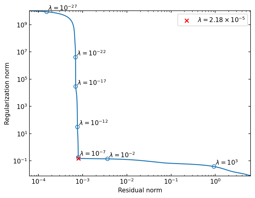
The L-curve shown above is limited to the range of \(\lambda\) from \(\sigma_0^2\) to \(\sigma_{r}^2\) and it is enough to find the corner of the L-curve in this range.

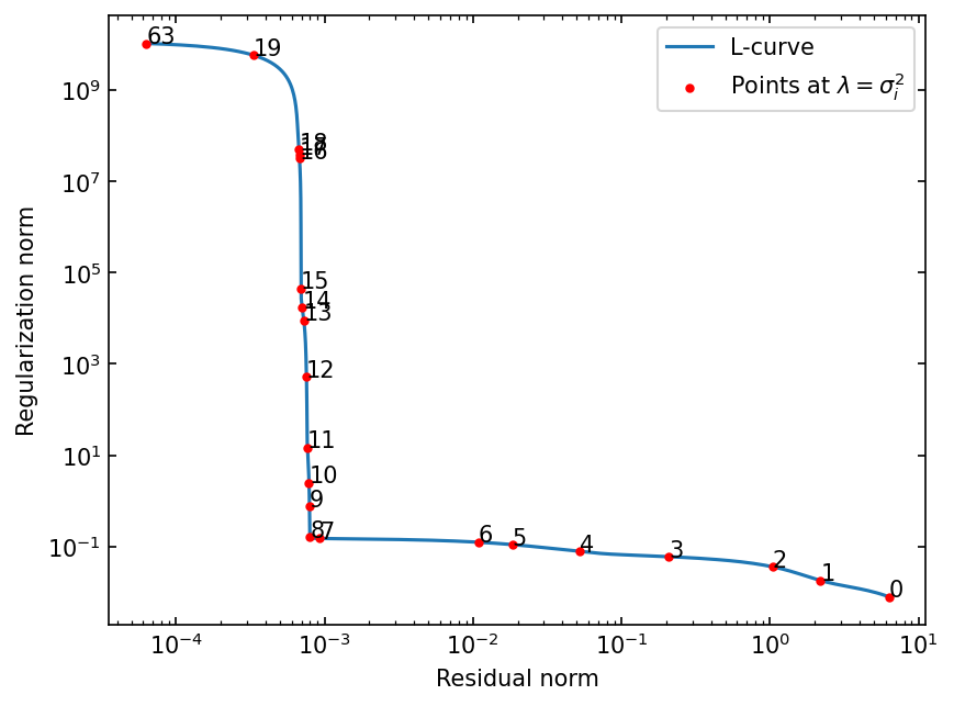
The below plot shows why it is enough by plotting points of \(\lambda = \sigma_i^2\) on the L-curve, where \(\sigma_i\) is the \(i\)-th singular value and \(i\) is indicated by the annotation.

fig, ax = lcurve.plot_L_curve(plot_lambda_opt=False)

indices = list(range(0, 20)) + [lcurve.s.size - 1]
sigmas = lcurve.s[indices]
residuals = [lcurve.residual_norm(beta) for beta in sigmas**2]
regularizations = [lcurve.regularization_norm(beta) for beta in sigmas**2]
ax.scatter(residuals, regularizations, color="red", marker=".")
ax.legend(["L-curve", "Points at $\\lambda = \\sigma_i^2$"])
for i, ind in enumerate(indices):
    ax.annotate(f"{ind}", (residuals[i], regularizations[i]))

print(f"sigma_7^2 : {sigmas[7]**2:.4e}")
print(f"sigma_8^2 : {sigmas[8]**2:.4e}")
print(f"sigma_9^2 : {sigmas[9]**2:.4e}")
print(f"lambda_opt: {lcurve.lambda_opt:.4e}")

sigma_7^2 : 6.4611e-04
sigma_8^2 : 1.2423e-06
sigma_9^2 : 4.5937e-09
lambda_opt: 2.1786e-05

Plot L-curve’s curvature

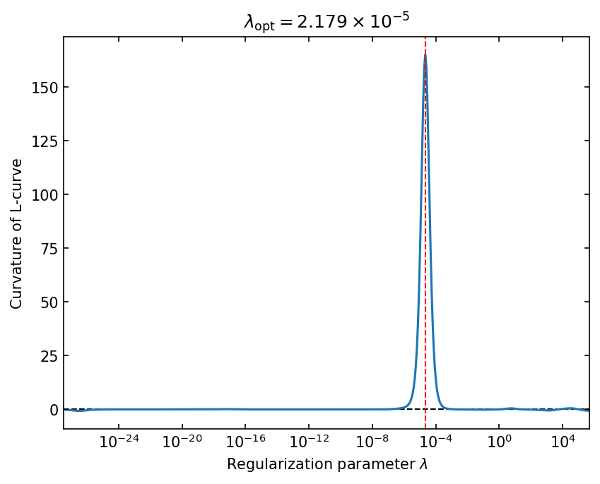
\(\lambda_\mathrm{opt}\) is the regularization parameter that maximizes the curvature of the L-curve.

_, ax = lcurve.plot_curvature()
lambda_opt_text = parse_scientific_notation(f"{lcurve.lambda_opt:.3e}")
ax.set_title(f"$\\lambda_\\mathrm{{opt}} = {lambda_opt_text}$")
ax.tick_params(axis="both", which="both", direction="in", top=True, right=True)

Compare \(\mathbf{x}_\lambda\) with \(\mathbf{x}_\mathrm{true}\)

Let us compare solutions at different regularization parameters \(\lambda=10^{-9}\), \(\lambda_\text{opt}\), \(10^3\) with the true solution \(\mathbf{x}_\mathrm{true}\).

lambdas = [1.0e-9, lcurve.lambda_opt, 1.0e3]

fig, axes = plt.subplots(1, 3, figsize=(10, 4), sharey=True, layout="constrained")

for ax, beta in zip(axes, lambdas, strict=False):
    ax.plot(t, x_t, "--", label="$\\mathbf{x}_\\mathrm{true}$")
    ax.plot(t, lcurve.solution(beta=beta), label="$\\mathbf{x}_\\lambda$")

    ax.set_xlim(t.min(), t.max())
    ax.set_ylim(0, x_t.max() * 1.1)
    ax.set_xlabel("$t$")
    parsed_lambda = parse_scientific_notation(f"{beta:.2e}")
    ax.set_title(f"$\\lambda = {parsed_lambda}$")
    ax.tick_params(direction="in", labelsize=10, which="both", top=True, right=True)
    ax.legend(loc="upper left")

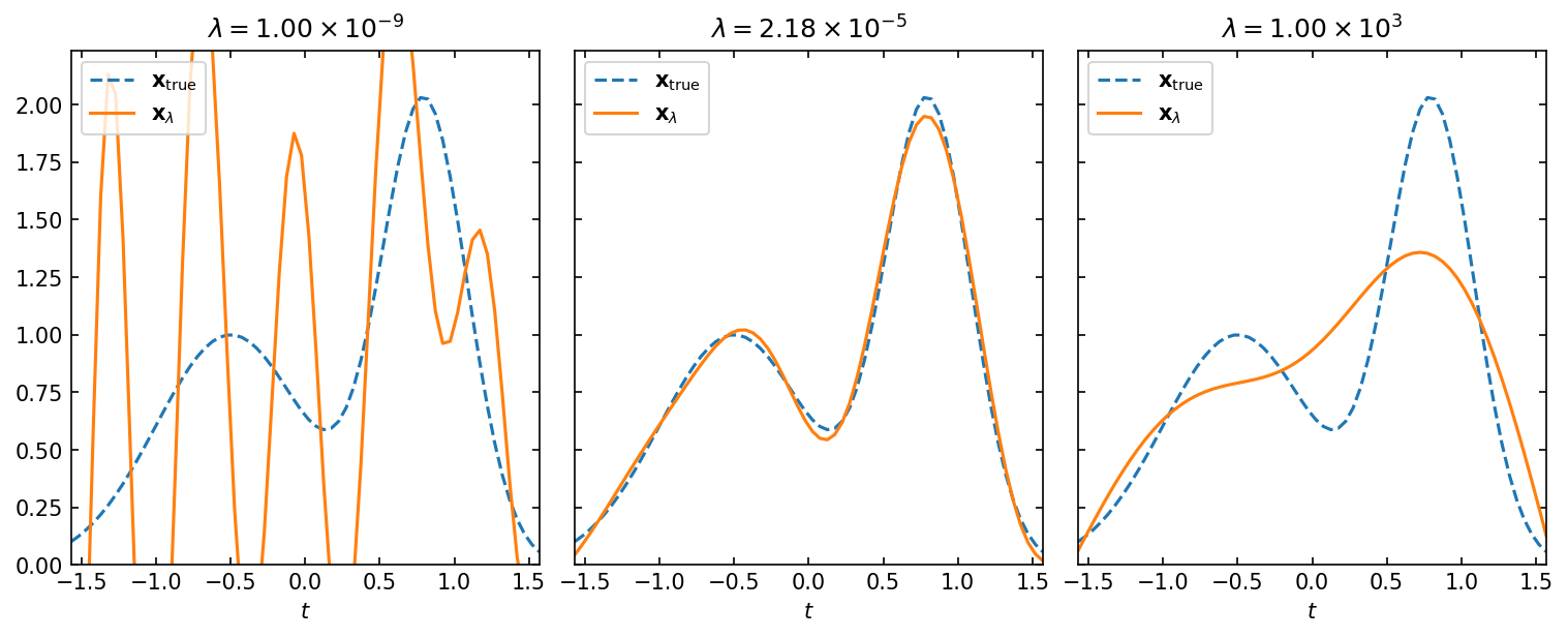
We can see that the solution at \(\lambda < \lambda_\mathrm{opt}\) is perturbed by noise, while the solution at \(\lambda > \lambda_\mathrm{opt}\) is smoothed too much.

Plot norms and curvature as a function of \(\lambda\)

Let us plot the residual norm \(\sqrt{\rho}\) and the regularization norm \(\sqrt{\eta}\) as a function of \(\lambda\). Additionally, we plot the curvature of the L-curve as a function of \(\lambda\).

fig, ax1 = plt.subplots()
fig.subplots_adjust(right=0.85)

ax2 = ax1.twinx()
ax3 = ax1.twinx()

ax3.spines.right.set_position(("axes", 1.2))

# calculation of the values
lambdas = np.logspace(-10, 0, num=500)
rhos = [lcurve.residual_norm(beta) for beta in lambdas]
etas = [lcurve.regularization_norm(beta) for beta in lambdas]
kappa = [lcurve.curvature(beta) for beta in lambdas]

# plot lines
(p1,) = ax1.loglog(lambdas, rhos, color="C0")
(p2,) = ax2.loglog(lambdas, etas, color="C1")
(p3,) = ax3.semilogx(lambdas, kappa, color="C2")

# set axes properties
ax1.set(
    xlim=(lambdas[0], lambdas[-1]),
    xlabel="Regularization parameter $\\lambda$",
    ylabel="Residual norm $\\sqrt{\\rho}$",
)
ax2.set(ylabel="Regularization norm $\\sqrt{\\eta}$")
ax3.set(ylabel="curvature of L-curve")

ax1.yaxis.label.set_color(p1.get_color())
ax2.yaxis.label.set_color(p2.get_color())
ax3.yaxis.label.set_color(p3.get_color())

ax1.tick_params(axis="x", which="both", direction="in", top=True)
ax1.tick_params(axis="y", which="both", direction="in", colors=p1.get_color())
ax2.tick_params(axis="y", which="both", direction="in", colors=p2.get_color())
ax3.tick_params(axis="y", which="both", direction="in", colors=p3.get_color())

ax3.spines["left"].set_color(p1.get_color())
ax2.spines["right"].set_color(p2.get_color())
ax3.spines["right"].set_color(p3.get_color())

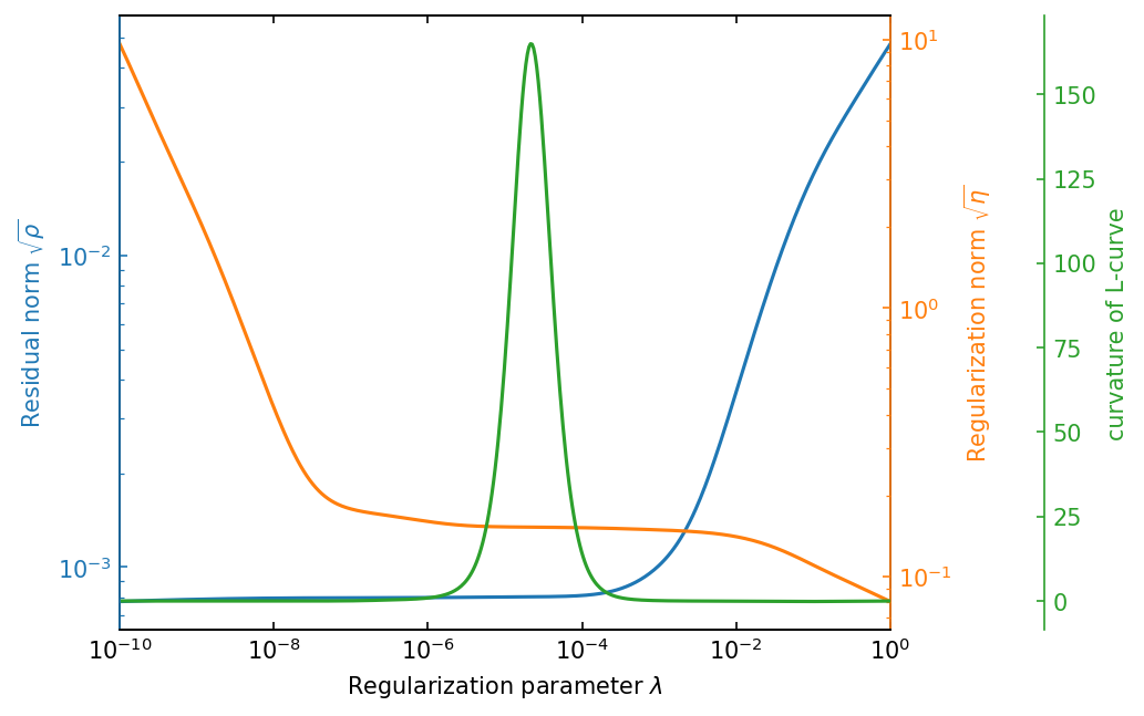
\(\sqrt{\rho}\) is monotonically increasing with \(\lambda\), while \(\sqrt{\eta}\) is monotonically decreasing with \(\lambda\). This behavior is consistent with the theory of the L-curve criterion.

The curvature of the L-curve is maximized at the center region where both are flat.

Check the relative error

The relative error between the solution \(\mathbf{x}_\lambda\) and the true solution \(\mathbf{x}_\mathrm{true}\) is defined as follows:

\[\begin{equation} \epsilon_\mathrm{rel} = \frac{\|\mathbf{x}_\lambda - \mathbf{x}_\mathrm{true}\|_2}{\|\mathbf{x}_\mathrm{true}\|_2}. \end{equation}\]

Let us seek the minimum \(\epsilon_\mathrm{rel}\) as a function of \(\lambda\).

from scipy.optimize import minimize_scalar

X_T_NORM = np.linalg.norm(x_t, axis=0)


def relative_error(
    log_lambda: float, x_t: np.ndarray = x_t, x_t_norm: float = X_T_NORM, lcurve: Lcurve = lcurve
) -> float:
    """Calculate relative error."""
    beta = 10**log_lambda
    sol = lcurve.solution(beta=beta)
    return np.linalg.norm(x_t - sol, axis=0) / x_t_norm


# minimize relative error
bounds = -10, -1
res = minimize_scalar(
    relative_error,
    bounds=bounds,
    method="bounded",
    args=(x_t, X_T_NORM, lcurve),
    options={"xatol": 1.0e-10, "maxiter": 1000},
)

# obtain minimum relative error and lambda
error_min = res.fun
lambda_min = 10**res.x

print(f"minimum relative error: {error_min:.2%} at lambda = {lambda_min:.4g}")

minimum relative error: 1.65% at lambda = 6.859e-07

Let us plot the relative error and curvature as a function of \(\lambda\).

# set regularization parameters
num = 500
lambdas = np.logspace(*bounds, num=num)

# calculate errors and curvatures
errors = np.asarray([relative_error(log_lambda) for log_lambda in np.linspace(*bounds, num=num)])
kappa = np.asarray([lcurve.curvature(beta) for beta in lambdas])

# create figure
fig, ax1 = plt.subplots()
ax2 = ax1.twinx()

# plot errors and curvatures
(p1,) = ax1.loglog(lambdas, errors, color="C0")
(p2,) = ax2.semilogx(lambdas, kappa, color="C1")

# plot minimum error vertical line and point
ax1.axvline(lambda_min, color="r", linestyle="--", linewidth=0.75)
ax1.scatter(lambda_min, error_min, color="r", marker="o", s=10, zorder=2)
ax1.text(
    lambda_min,
    1.5e-2,
    "$\\lambda_\\mathrm{min}$",
    color="r",
    horizontalalignment="left",
    verticalalignment="center",
)

# plot maximum curvature vertical line and point
assert lcurve.lambda_opt is not None
ax1.axvline(lcurve.lambda_opt, color="g", linestyle="--", linewidth=0.75)
ax2.scatter(
    lcurve.lambda_opt, lcurve.curvature(lcurve.lambda_opt), color="g", marker="o", s=10, zorder=2
)
ax1.text(
    lcurve.lambda_opt,
    1.5e-2,
    "$\\lambda_\\mathrm{opt}$",
    color="g",
    horizontalalignment="left",
    verticalalignment="center",
)

# set axes
ax1.set(
    xlim=(lambdas[0], lambdas[-1]),
    ylim=(0.01, 1),
    xlabel="$\\lambda$",
    ylabel="Relative error $\\epsilon_\\mathrm{rel}$",
)
ax2.set(ylabel="curvature of L-curve")

ax1.yaxis.label.set_color(p1.get_color())
ax2.yaxis.label.set_color(p2.get_color())

ax1.tick_params(axis="x", which="both", direction="in", top=True)
ax1.tick_params(axis="y", which="both", direction="in", colors=p1.get_color())
ax2.tick_params(axis="y", which="both", direction="in", colors=p2.get_color())

ax2.spines["left"].set_color(p1.get_color())
ax2.spines["right"].set_color(p2.get_color())

error_opt = relative_error(np.log10(lcurve.lambda_opt))
ax1.set_title(
    f"$\\epsilon_\\mathrm{{rel}}(\\lambda_\\mathrm{{opt}})$ = {error_opt:.2%}, "
    + f"$\\epsilon_\\mathrm{{rel}}(\\lambda_\\mathrm{{min}}) = ${error_min:.2%}"
);

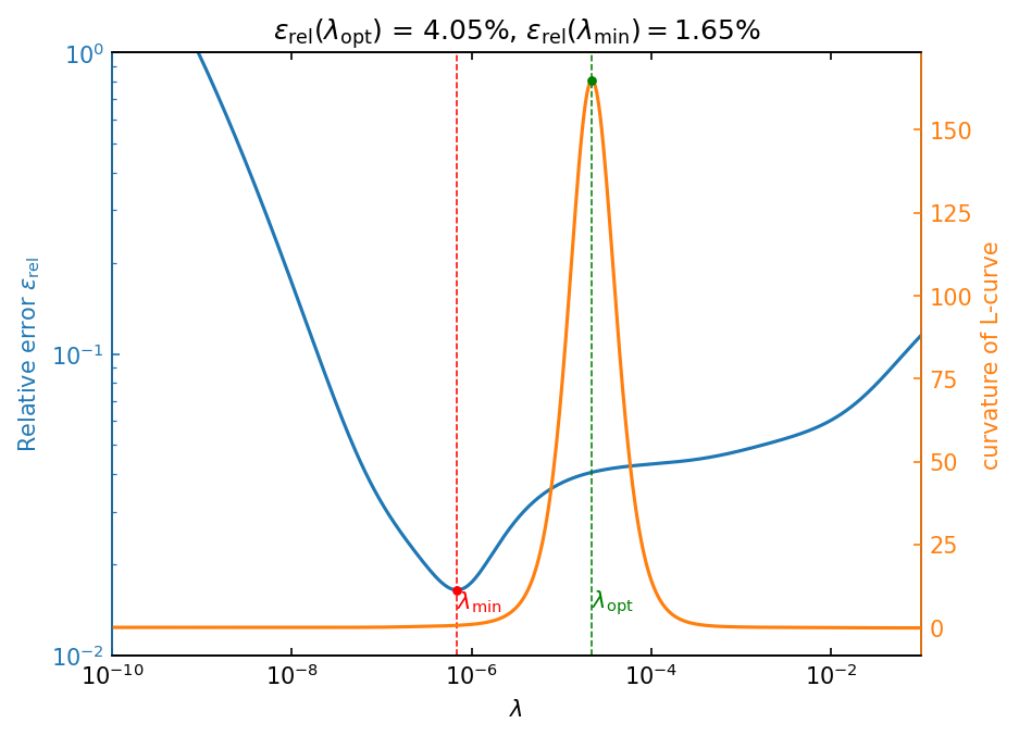
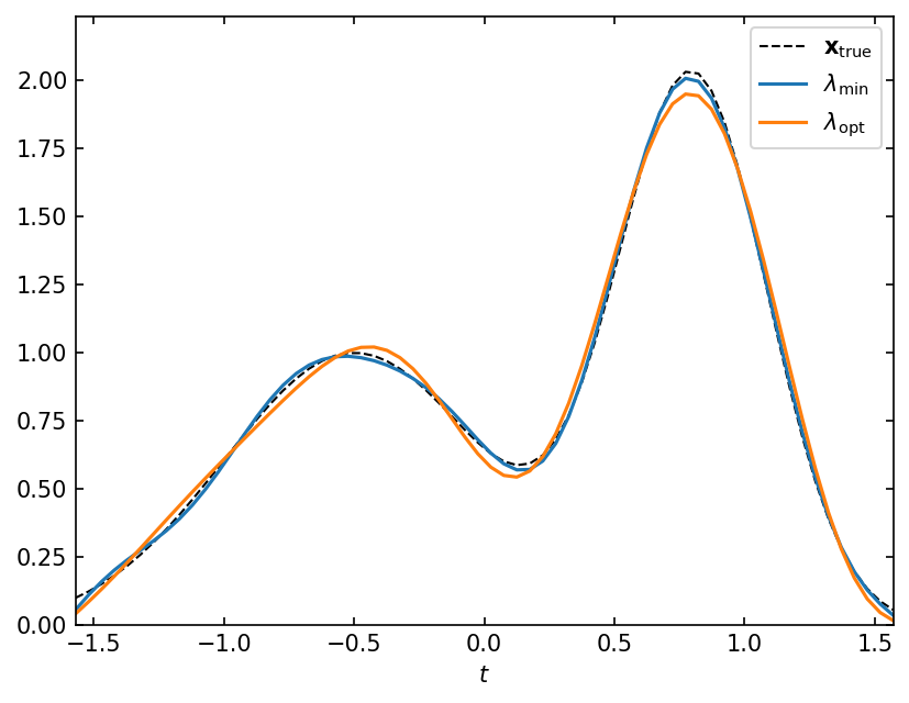
Compare the solution at \(\lambda_\mathrm{opt}\) with \(\lambda_\mathrm{min}\)

\(\lambda_\mathrm{min}\) is the regularization parameter that minimizes the relative error.

fig, ax = plt.subplots()
ax.plot(t, x_t, "k--", label="$\\mathbf{x}_\\mathrm{true}$", linewidth=1.0)
ax.plot(t, lcurve.solution(lambda_min), label="$\\lambda_\\mathrm{min}$")
ax.plot(t, sol, label="$\\lambda_\\mathrm{opt}$")
ax.set_xlabel("$t$")
ax.set_xlim(t.min(), t.max())
ax.set_ylim(0, x_t.max() * 1.1)
ax.legend()
ax.tick_params(axis="both", which="both", direction="in", top=True, right=True)

Discrete Picard Plot

Discrete Picard Condition[1]

The data vector \(\mathbf{b}\) satisfies the discrete Picard condition (DPC) if the data space coefficients \(|\mathbf{u}_i^\mathsf{T}\mathbf{b}|\) decay faster than the singular values \(\sigma_i\).

In ill-posed problems, we find that the DPC holds initially and then fails at some point \(i_\mathrm{DPC}\), where the data become dominated by errors (noise). If this is the case, and if the regularization parameter is accurately selected, then the regularized solution should provide a valid solution. Examining \(i_\mathrm{DPC}\) provides a method of characterizing the ill-posedness of the problem.

ub = np.abs(lcurve.U.T @ b)

fig, ax1 = plt.subplots()
ax2 = ax1.twinx()

# DP plot
ax1.semilogy(lcurve.s, ".-", label="$\\sigma_i$")
ax1.semilogy(ub, "o", label="$|\\mathbf{u}_i^\\mathsf{T}\\mathbf{b}|$")
ax1.semilogy(ub / lcurve.s, "s", label="$|\\mathbf{u}_i^\\mathsf{T}\\mathbf{b}|/\\sigma_i$")
ax1.axhline(1e-4, color="k", linestyle="--", zorder=0)
ax1.axvline(10, color="k", linestyle="--", zorder=0)
ax1.set_xlabel("$i$")
ax1.legend(loc="lower left")
ax1.tick_params(axis="both", which="both", direction="in", top=True)

# filter plot
assert lcurve.lambda_opt is not None
(p2,) = ax2.semilogy(
    lcurve.filter(lcurve.lambda_opt), ".-", color="C4", label="$\\mathbf{f}_\\mathrm{opt}$"
)
ax2.set_ylabel("$f_{\\lambda, i}$", color="C4")

# color axes2
ax2.yaxis.label.set_color(p2.get_color())
ax2.tick_params(axis="y", which="both", direction="in", colors=p2.get_color())
ax2.spines["right"].set_color(p2.get_color())

ax1.set_xlim(0, 25);

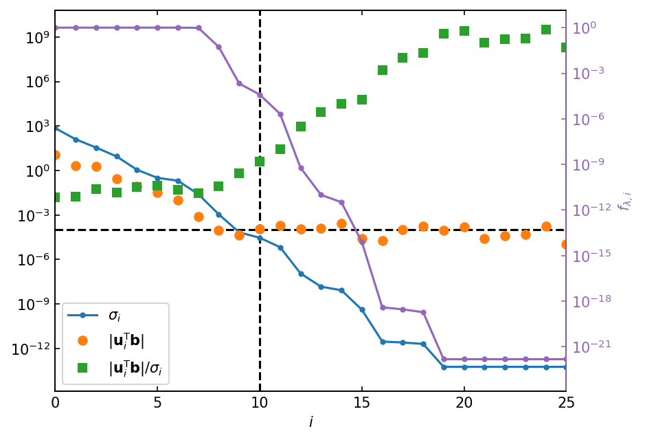
The vertical dashed line in the above figure marks the biginning of \(|\mathbf{u}_i^\mathsf{T}\mathbf{b}| < \sigma_i\), and the horizontal dashed line represents the noise level. DPC is satisfied for \(i < i_\mathrm{DPC} \simeq 10\). We confirm that the filter factor \(f_{\lambda_\mathrm{opt}, i}\), the \(\lambda_\mathrm{opt}\) of which is selected by the L-curve criterion, starts to decrease around \(i_\mathrm{DPC}\). This behavior works as a filter to suppress the noise component and yields a physically meaningful solution.

References

[1]

Teresa Correia, Adam Gibson, Martin Schweiger, and Jeremy Hebden. Selection of regularization parameter for optical topography. J. Biomed. Opt., 14(3):034044, 2009. doi:10.1117/1.3156839.