Note

This page was generated from notebooks/non-iterative/lcurve_vs_gcv.ipynb.

Analysis of discrete ill-posed problem with different types of noise

This notebook is aimed at analyzing the behavior of different regularization methods for discrete ill-posed problems with different types of noise. The referenced papare is [1].

import numpy as np
from matplotlib import pyplot as plt
from scipy.optimize import minimize_scalar
from scipy.sparse import diags

from cherab.inversion import GCV, Lcurve, _SVDBase, compute_svd
from cherab.inversion.tools import parse_scientific_notation

plt.rcParams["figure.dpi"] = 150
plt.rcParams["figure.constrained_layout.use"] = True

Definition of the example problem

Let us consider the following kernel and solution function derived from the Fredholm intgral equation of the first kind:

\[\begin{split}\begin{align} K(s, t) &\equiv \left( \cos(s) + \cos(t) \right)^2 \left( \frac{\sin \psi(s, t)}{\psi(s, t)} \right)^2,\quad \psi(s, t)\equiv\pi\left(\sin(s) + \sin(t)\right)\\ x(t) &\equiv 2.0\exp(-4(t-0.5)^2) + \exp(-4(t+0.5)^2) \end{align}\end{split}\]

def _func(s: float, t: float) -> float:
    return np.pi * (np.sin(s) + np.sin(t))


def kernel(s: float, t: float) -> float:
    """The kernel function."""
    u = _func(s, t)
    if u == 0:
        return (np.cos(s) + np.cos(t)) ** 2.0
    else:
        return ((np.cos(s) + np.cos(t)) * np.sin(u) / u) ** 2.0


def solution(t: float) -> float:
    """The solution function."""
    return 2.0 * np.exp(-4.0 * (t - 0.5) ** 2.0) + np.exp(-4.0 * (t + 0.5) ** 2.0)

Discrete \(s\) and \(t\) in the range \(\displaystyle\left[-\frac{\pi}{2}, \frac{\pi}{2}\right]\) are used and the noise-free data \(\bar{\mathbf{b}}\) is given by \(\bar{\mathbf{b}} = \mathbf{K}\mathbf{x}\).

s = np.linspace(-0.5 * np.pi, 0.5 * np.pi, num=64, endpoint=True)
t = np.linspace(-0.5 * np.pi, 0.5 * np.pi, num=64, endpoint=True)

# discretize kernel
k_mat = np.zeros((s.size, t.size))
k_mat = np.array([[kernel(i, j) for j in t] for i in s])

# trapezoidal rule
k_mat[:, 0] *= 0.5
k_mat[:, -1] *= 0.5
k_mat *= t[1] - t[0]

# discretize solution
x_t = np.array([solution(i) for i in t])

# noise-free data
b_bar = k_mat @ x_t

print(f"{k_mat.shape = }")
print(f"{x_t.shape = }")
print(f"condition number of K is {np.linalg.cond(k_mat):.4g}")

k_mat.shape = (64, 64)
x_t.shape = (64,)
condition number of K is 2.04e+18

Perturbation by wite noise

First we consider the case of uncorrelated errors (white nise), i.e., the elements \(e_i\) of the purturbation \(\mathbf{e}\) are normally distributed with zero mean and standard deviation \(10^{-3}\). Hence the right-hand side \(\mathbf{b}\) of the perturbed problem is given by \(\mathbf{b} = \bar{\mathbf{b}} + \mathbf{e}\).

rng = np.random.default_rng()
noise = rng.normal(0, 1.0e-3, b_bar.size)
b = b_bar + noise

The solution \(\mathbf{x}_\lambda = \left(\mathbf{K}^\mathsf{T}\mathbf{K} + \lambda\mathbf{I}\right)^{-1}\mathbf{K}^\mathsf{T}\mathbf{b}\) is computed and opimized for the regularization parameter \(\lambda\) using the GCV and L-curve criteria.

# Compute SVD using K & I matrices
Imat = diags([1], shape=(t.size, t.size))
s, u, basis = compute_svd(k_mat, Imat)

# create GCV and L-curve objects
gcv = GCV(s, u, basis, data=b)
lcurve = Lcurve(s, u, basis, data=b)

# solve for the regularization parameter
sol_gcv, _ = gcv.solve()
sol_lcurve, _ = lcurve.solve()

Show the L-curve’s curvature and the GCV as a function of \(\lambda\).

fig, axes = plt.subplots(1, 2, figsize=(10, 5))
lcurve.plot_curvature(fig=fig, axes=axes[0])
gcv.plot_gcv(fig=fig, axes=axes[1])
lambda_opt_lcurve = parse_scientific_notation(f"{lcurve.lambda_opt:.2e}")
lambda_opt_gcv = parse_scientific_notation(f"{gcv.lambda_opt:.2e}")
axes[0].set_title(f"L-curve curvature ($\\lambda_\\mathrm{{opt}} = {lambda_opt_lcurve}$)")
axes[1].set_title(f"GCV ($\\lambda_\\mathrm{{opt}} = {lambda_opt_gcv}$)");

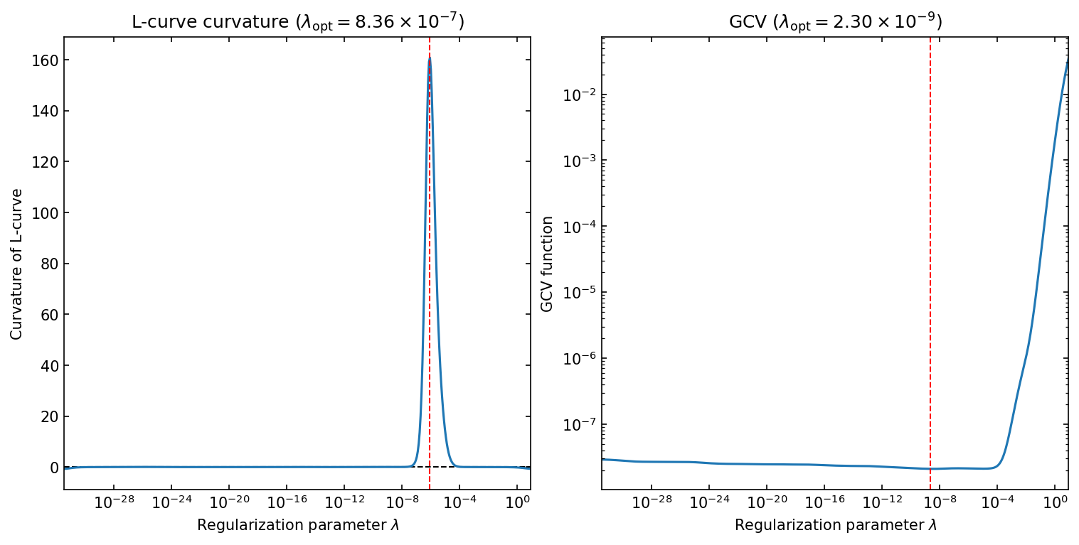
Let us calculate the relative error for each optimal solution and compare the results.

X_T_NORM = np.linalg.norm(x_t, axis=0)


def relative_error(
    log_lambda: float,
    x_t: np.ndarray = x_t,
    x_t_norm: float = X_T_NORM,
    regularizer: _SVDBase = lcurve,
) -> float:
    """Calculate relative error."""
    beta = 10**log_lambda
    sol = regularizer.solution(beta=beta)
    return np.linalg.norm(x_t - sol, axis=0) / x_t_norm


# minimize relative error
bounds = (-40, 0)
res = minimize_scalar(
    relative_error,
    bounds=bounds,
    method="bounded",
    args=(x_t, X_T_NORM, gcv),
    options={"xatol": 1.0e-10, "maxiter": 1000},
)

# obtain minimum relative error and lambda
error_min = res.fun
lambda_min = 10**res.x

print("          Regularization Parameter   Relative Error")
print("          ------------------------  ----------------")
print(f"GCV       {gcv.lambda_opt:^27.4e}  {relative_error(np.log10(gcv.lambda_opt)):^12.4%}")
print(f"L-curve   {lcurve.lambda_opt:^27.4e}  {relative_error(np.log10(lcurve.lambda_opt)):^12.4%}")
print(f"Min Error {lambda_min:^27.4e}  {error_min:^12.4%}")

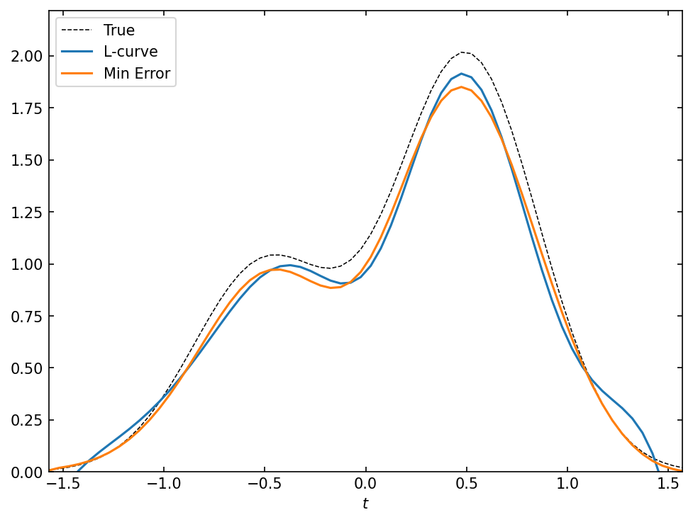
          Regularization Parameter   Relative Error
          ------------------------  ----------------
GCV               2.3005e-09            208.0212%
L-curve           8.3555e-07             8.6321%
Min Error         5.2299e-05             1.2472%

Each optimal solution is plotted together with the original solution and the minimum-error one.

sols = [sol_gcv, sol_lcurve, lcurve.solution(beta=lambda_min)]
labels = ["GCV", "L-curve", "Min Error"]

fig, ax = plt.subplots()
ax.plot(t, x_t, ls="--", lw=0.75, color="k", label="True")
for sol, label in zip(sols, labels, strict=False):
    ax.plot(t, sol, label=label)

ax.set_xlim(t.min(), t.max())
ax.set_ylim(0, x_t.max() * 1.1)
ax.set_xlabel("$t$")
ax.tick_params(direction="in", labelsize=10, which="both", top=True, right=True)
ax.legend(loc="upper left");

Purturbation by uncorrelated noise

Next we consider the case of highly correlated errors, which are derived from a regular smoothing of the matrix \(\mathbf{K}\) and the right-hand side \(\bar{\mathbf{b}}\):

\[\begin{split}\begin{align} \tilde{\mathbf{K}}_{i,j} &\equiv \mathbf{K}_{i,j} + \mu \left( \mathbf{K}_{i,j-1} + \mathbf{K}_{i,j+1} + \mathbf{K}_{i-1,j} + \mathbf{K}_{i+1,j} \right),\\ \tilde{\mathbf{b}}_i &\equiv \bar{\mathbf{b}}_i + \mu \left( \bar{\mathbf{b}}_{i-1} + \bar{\mathbf{b}}_{i+1} \right), \end{align}\end{split}\]

where \(\mu\) is set to \(0.05\) and the outside elements are set to zero.

mu = 0.05

k_mat_smooth = np.zeros_like(k_mat)
b = np.zeros_like(b_bar)

for i in range(len(b_bar)):
    if i < 1:
        b[i] = b_bar[i] + mu * (0 + b_bar[i + 1])
    elif i > len(b_bar) - 2:
        b[i] = b_bar[i] + mu * (b_bar[i - 1] + 0)
    else:
        b[i] = b_bar[i] + mu * (b_bar[i - 1] + b_bar[i + 1])


for i in range(k_mat.shape[0]):
    for j in range(k_mat.shape[1]):
        if i - 1 < 0:
            k1 = 0
        else:
            k1 = k_mat[i - 1, j]
        if i + 1 > k_mat.shape[0] - 1:
            k2 = 0
        else:
            k2 = k_mat[i + 1, j]
        if j - 1 < 0:
            k3 = 0
        else:
            k3 = k_mat[i, j - 1]
        if j + 1 > k_mat.shape[1] - 1:
            k4 = 0
        else:
            k4 = k_mat[i, j + 1]

        k_mat_smooth[i, j] = k_mat[i, j] + mu * (k1 + k2 + k3 + k4)

We solve the perturbed problem with the same regularization methods and plot both criteria as a function of \(\lambda\).

# Compute SVD using K & I matrices
s, u, basis = compute_svd(k_mat_smooth, Imat)

# create GCV and L-curve objects
gcv = GCV(s, u, basis, data=b)
lcurve = Lcurve(s, u, basis, data=b)

# solve for the regularization parameter
sol_gcv, _ = gcv.solve()
sol_lcurve, _ = lcurve.solve()

# plot the L-curve's curvature and GCV
fig, axes = plt.subplots(1, 2, figsize=(10, 5))
lcurve.plot_curvature(fig=fig, axes=axes[0])
gcv.plot_gcv(fig=fig, axes=axes[1])
lambda_opt_lcurve = parse_scientific_notation(f"{lcurve.lambda_opt:.2e}")
lambda_opt_gcv = parse_scientific_notation(f"{gcv.lambda_opt:.2e}")
axes[0].set_title(f"L-curve curvature ($\\lambda_\\mathrm{{opt}} = {lambda_opt_lcurve}$)")
axes[1].set_title(f"GCV ($\\lambda_\\mathrm{{opt}} = {lambda_opt_gcv}$)");

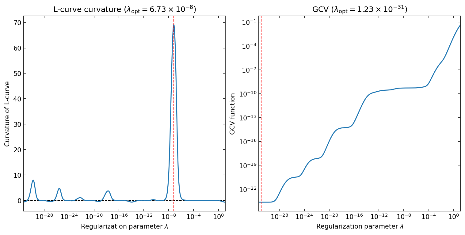
The L-curve method still works well by finding the corner of the L-curve, however, the GCV method fails to find the minimum of the GCV function in the same range of \(\lambda\).

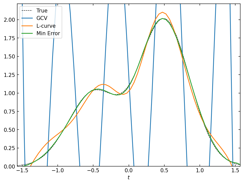
Let us calculate relative errors and plot the optimal solutions as well as the original solution and the minimum-error one.

# minimize relative error
bounds = (-20, 0)
res = minimize_scalar(
    relative_error,
    bounds=bounds,
    method="bounded",
    args=(x_t, X_T_NORM, gcv),
    options={"xatol": 1.0e-10, "maxiter": 1000},
)

# obtain minimum relative error and lambda
error_min = res.fun
lambda_min = 10**res.x

print("          Regularization Parameter   Relative Error")
print("          ------------------------  ----------------")
print(f"GCV       {gcv.lambda_opt:^27.4e}  {relative_error(np.log10(gcv.lambda_opt)):^12.4%}")
print(f"L-curve   {lcurve.lambda_opt:^27.4e}  {relative_error(np.log10(lcurve.lambda_opt)):^12.4%}")
print(f"Min Error {lambda_min:^27.4e}  {error_min:^12.4%}")

          Regularization Parameter   Relative Error
          ------------------------  ----------------
GCV               1.2253e-31           102514588967553.6250%
L-curve           6.7347e-08             28.1151%
Min Error         2.8872e-05             8.4945%

sols = [sol_lcurve, lcurve.solution(beta=lambda_min)]
labels = ["L-curve", "Min Error"]

fig, ax = plt.subplots()
ax.plot(t, x_t, ls="--", lw=0.75, color="k", label="True")
for sol, label in zip(sols, labels, strict=False):
    ax.plot(t, sol, label=label)

ax.set_xlim(t.min(), t.max())
ax.set_ylim(0, x_t.max() * 1.1)
ax.set_xlabel("$t$")
ax.tick_params(direction="in", labelsize=10, which="both", top=True, right=True)
ax.legend(loc="upper left");

References

[1]

Per Christian Hansen. Analysis of discrete ill-posed problems by means of the L-curve. SIAM Rev., 34(4):561–580, 1992. doi:10.1137/1034115.