Note
This page was generated from notebooks/others/derivative_operator.ipynb.
Derivative Operation#
Here we show you examples of derivative/laplacian matrices and how they work on the example image.
Please see the derivative theory page if you want to know the details of the theory.
[1]:
import numpy as np
from matplotlib import pyplot as plt
from matplotlib.cbook import get_sample_data
from matplotlib.cm import ScalarMappable
from matplotlib.colors import CenteredNorm
from mpl_toolkits.axes_grid1 import ImageGrid
from PIL import Image

from cherab.inversion.derivative import derivative_matrix, laplacian_matrix
Visualize derivative matrix#
Let us compute the simple derivative matrix applying a 3 x 3 image array.
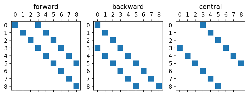
Firstly we show derivative matrices along to vertical direction (axis=0 direction) with different schemes. The derivative matrices are shown by printing the matrix elements and plotting the matrix elements in 2-D image. The blue squares represent the matrix elements.
[2]:
fig, axes = plt.subplots(1, 3, dpi=150, tight_layout=True)
for ax, scheme in zip(axes, ["forward", "backward", "central"]):  # noqa
    # compute derivative matrix
    dmat = derivative_matrix((3, 3), axis=0, scheme=scheme)

    # print array
    print(f"Derivative matrix ({scheme}):\n{dmat.toarray()}\n")

    # plot derivative matrix as a sparse one
    ax.spy(dmat)
    ax.set_title(f"{scheme}")
Derivative matrix (forward):
[[-1.  0.  0.  1.  0.  0.  0.  0.  0.]
 [ 0. -1.  0.  0.  1.  0.  0.  0.  0.]
 [ 0.  0. -1.  0.  0.  1.  0.  0.  0.]
 [ 0.  0.  0. -1.  0.  0.  1.  0.  0.]
 [ 0.  0.  0.  0. -1.  0.  0.  1.  0.]
 [ 0.  0.  0.  0.  0. -1.  0.  0.  1.]
 [ 0.  0.  0.  0.  0.  0. -1.  0.  0.]
 [ 0.  0.  0.  0.  0.  0.  0. -1.  0.]
 [ 0.  0.  0.  0.  0.  0.  0.  0. -1.]]

Derivative matrix (backward):
[[ 1.  0.  0.  0.  0.  0.  0.  0.  0.]
 [ 0.  1.  0.  0.  0.  0.  0.  0.  0.]
 [ 0.  0.  1.  0.  0.  0.  0.  0.  0.]
 [-1.  0.  0.  1.  0.  0.  0.  0.  0.]
 [ 0. -1.  0.  0.  1.  0.  0.  0.  0.]
 [ 0.  0. -1.  0.  0.  1.  0.  0.  0.]
 [ 0.  0.  0. -1.  0.  0.  1.  0.  0.]
 [ 0.  0.  0.  0. -1.  0.  0.  1.  0.]
 [ 0.  0.  0.  0.  0. -1.  0.  0.  1.]]

Derivative matrix (central):
[[ 0.   0.   0.   0.5  0.   0.   0.   0.   0. ]
 [ 0.   0.   0.   0.   0.5  0.   0.   0.   0. ]
 [ 0.   0.   0.   0.   0.   0.5  0.   0.   0. ]
 [-0.5  0.   0.   0.   0.   0.   0.5  0.   0. ]
 [ 0.  -0.5  0.   0.   0.   0.   0.   0.5  0. ]
 [ 0.   0.  -0.5  0.   0.   0.   0.   0.   0.5]
 [ 0.   0.   0.  -0.5  0.   0.   0.   0.   0. ]
 [ 0.   0.   0.   0.  -0.5  0.   0.   0.   0. ]
 [ 0.   0.   0.   0.   0.  -0.5  0.   0.   0. ]]
Also we show the horizontal derivative matrix (axis=1 direction) case.
[3]:
fig, axes = plt.subplots(1, 3, dpi=150, tight_layout=True)
for ax, scheme in zip(axes, ["forward", "backward", "central"]):  # noqa
    # compute derivative matrix
    dmat = derivative_matrix((3, 3), axis=1, scheme=scheme)

    # print array
    print(f"Derivative matrix ({scheme}):\n{dmat.toarray()}\n")

    # plot derivative matrix as a sparse one
    ax.spy(dmat)
    ax.set_title(f"{scheme}")
Derivative matrix (forward):
[[-1.  1.  0.  0.  0.  0.  0.  0.  0.]
 [ 0. -1.  1.  0.  0.  0.  0.  0.  0.]
 [ 0.  0. -1.  0.  0.  0.  0.  0.  0.]
 [ 0.  0.  0. -1.  1.  0.  0.  0.  0.]
 [ 0.  0.  0.  0. -1.  1.  0.  0.  0.]
 [ 0.  0.  0.  0.  0. -1.  0.  0.  0.]
 [ 0.  0.  0.  0.  0.  0. -1.  1.  0.]
 [ 0.  0.  0.  0.  0.  0.  0. -1.  1.]
 [ 0.  0.  0.  0.  0.  0.  0.  0. -1.]]

Derivative matrix (backward):
[[ 1.  0.  0.  0.  0.  0.  0.  0.  0.]
 [-1.  1.  0.  0.  0.  0.  0.  0.  0.]
 [ 0. -1.  1.  0.  0.  0.  0.  0.  0.]
 [ 0.  0.  0.  1.  0.  0.  0.  0.  0.]
 [ 0.  0.  0. -1.  1.  0.  0.  0.  0.]
 [ 0.  0.  0.  0. -1.  1.  0.  0.  0.]
 [ 0.  0.  0.  0.  0.  0.  1.  0.  0.]
 [ 0.  0.  0.  0.  0.  0. -1.  1.  0.]
 [ 0.  0.  0.  0.  0.  0.  0. -1.  1.]]

Derivative matrix (central):
[[ 0.   0.5  0.   0.   0.   0.   0.   0.   0. ]
 [-0.5  0.   0.5  0.   0.   0.   0.   0.   0. ]
 [ 0.  -0.5  0.   0.   0.   0.   0.   0.   0. ]
 [ 0.   0.   0.   0.   0.5  0.   0.   0.   0. ]
 [ 0.   0.   0.  -0.5  0.   0.5  0.   0.   0. ]
 [ 0.   0.   0.   0.  -0.5  0.   0.   0.   0. ]
 [ 0.   0.   0.   0.   0.   0.   0.   0.5  0. ]
 [ 0.   0.   0.   0.   0.   0.  -0.5  0.   0.5]
 [ 0.   0.   0.   0.   0.   0.   0.  -0.5  0. ]]
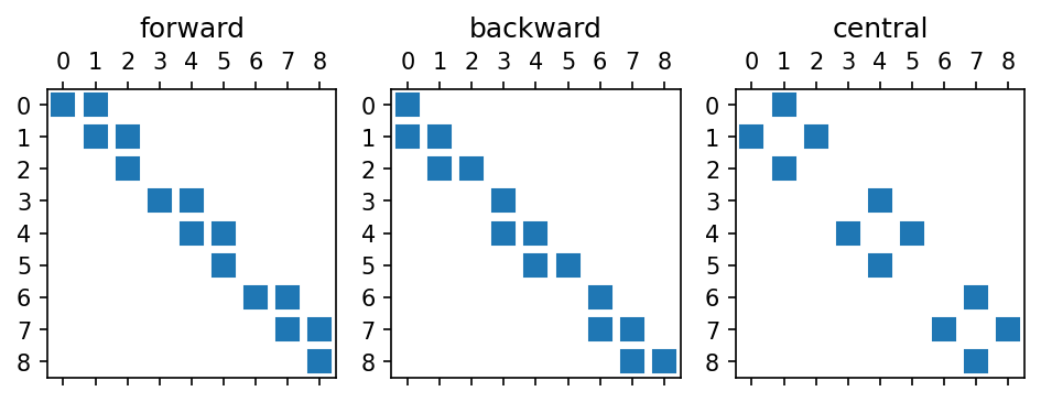
We can see that some elements are zero due to the boundary condition.
Visualize laplacian matrix#
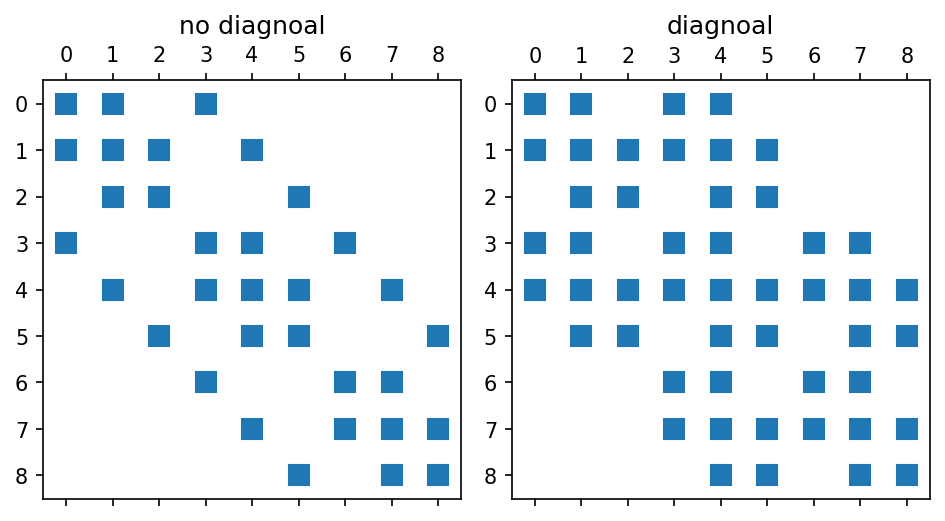
Let us compute the simple laplacian matrix applying a 3 x 3 image array and show it by printing the matrix elements and plotting the matrix elements in 2-D image. There are two types of laplacian matrix: difference between only orthogonal neighbors or all neighbors including diagonal neighbors. The step size along diagonal direction is \(\sqrt{2}h\).
[4]:
fig, axes = plt.subplots(1, 2, dpi=150, tight_layout=True)
for ax, diagonal in zip(axes, [False, True]):  # noqa
    # compute laplacian matrix
    lmat = laplacian_matrix((3, 3), diagonal=diagonal)

    # plot laplacian matrix as a sparse one
    ax.spy(lmat)
    title = "diagnoal" if diagonal else "no diagnoal"
    ax.set_title(f"{title}")

    # print array
    print(f"Laplacian matrix with {title}:\n{lmat.toarray()}\n")
Laplacian matrix with no diagnoal:
[[-4.  1.  0.  1.  0.  0.  0.  0.  0.]
 [ 1. -4.  1.  0.  1.  0.  0.  0.  0.]
 [ 0.  1. -4.  0.  0.  1.  0.  0.  0.]
 [ 1.  0.  0. -4.  1.  0.  1.  0.  0.]
 [ 0.  1.  0.  1. -4.  1.  0.  1.  0.]
 [ 0.  0.  1.  0.  1. -4.  0.  0.  1.]
 [ 0.  0.  0.  1.  0.  0. -4.  1.  0.]
 [ 0.  0.  0.  0.  1.  0.  1. -4.  1.]
 [ 0.  0.  0.  0.  0.  1.  0.  1. -4.]]

Laplacian matrix with diagnoal:
[[-6.   1.   0.   1.   0.5  0.   0.   0.   0. ]
 [ 1.  -6.   1.   0.5  1.   0.5  0.   0.   0. ]
 [ 0.   1.  -6.   0.   0.5  1.   0.   0.   0. ]
 [ 1.   0.5  0.  -6.   1.   0.   1.   0.5  0. ]
 [ 0.5  1.   0.5  1.  -6.   1.   0.5  1.   0.5]
 [ 0.   0.5  1.   0.   1.  -6.   0.   0.5  1. ]
 [ 0.   0.   0.   1.   0.5  0.  -6.   1.   0. ]
 [ 0.   0.   0.   0.5  1.   0.5  1.  -6.   1. ]
 [ 0.   0.   0.   0.   0.5  1.   0.   1.  -6. ]]
Apply the derivative/laplacian matrix to a sample image#
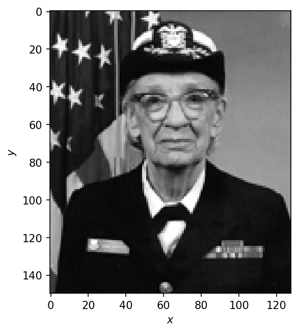
Next, let us to apply derivative/laplacian matrices to pixels of a sample image. We use sample image stored in matplotlib library.
Let us preview the sample image converted to monochrome image.
[5]:
with get_sample_data("grace_hopper.jpg") as file:
    arr_image = plt.imread(file)

# resize the image to 1/4 of the original size
with Image.fromarray(arr_image, mode="RGB") as im:
    (width, height) = (im.width // 4, im.height // 4)
    arr_image = np.array(im.resize((width, height)))

# convert RGB image to monotonic one
arr_image = arr_image.mean(axis=2)

# show image
print(f"image array shape: {arr_image.shape}")
fig, ax = plt.subplots(dpi=150)
im = ax.imshow(arr_image, cmap="gray")
ax.set_xlabel("$x$")
ax.set_ylabel("$y$");
image array shape: (150, 128)
Then create the derivative/laplacian matrices. Note that the \(x\), \(y\) directions correspond to the 1, 0 axis of the image array, respectively, and the positive direction of the \(y\) axis is downward.
[6]:
# compute each derivative matrix along each axis with forward scheme
dmat_x = derivative_matrix(arr_image.shape, axis=1, scheme="forward")
dmat_y = derivative_matrix(arr_image.shape, axis=0, scheme="forward")

# compute derivative matrices along y direction with different schemes
dmat_y_backward = derivative_matrix(arr_image.shape, axis=0, scheme="backward")
dmat_y_central = derivative_matrix(arr_image.shape, axis=0, scheme="central")

# compute laplacian matrices with and without diagonal
lmat_diag = laplacian_matrix(arr_image.shape, diagonal=True)
lmat_no_diag = laplacian_matrix(arr_image.shape, diagonal=False)
Check the difference effect of the derivative matrix between \(x\) and \(y\) directions#
[7]:
# compute derivative of images
arr_derivatives = []
vmax = 0
for dmat in [dmat_x, dmat_y]:
    arr_derivative = dmat @ arr_image.flatten()
    arr_derivative = arr_derivative.reshape(arr_image.shape)

    # retrieve abosolute maximum value of derivative and choose the largest one
    vmax = val if (val := np.abs(arr_derivative).max()) > vmax else vmax
    arr_derivatives.append(arr_derivative)

fig = plt.figure(dpi=150)
grids = ImageGrid(fig, 111, nrows_ncols=(1, 2), cbar_mode="single")
norm = CenteredNorm(halfrange=vmax)
for ax, arr, title in zip(grids, arr_derivatives, ["$x$", "$y$"]):  # noqa
    # plot derivative
    im = ax.imshow(arr, cmap="RdBu_r", norm=norm)
    ax.set_xlabel("$x$")
    ax.set_ylabel("$y$")
    ax.set_title(f"{title} direction")

# plot colorbar
mappable = ScalarMappable(norm=norm, cmap="RdBu_r")
cbar = plt.colorbar(mappable, cax=grids.cbar_axes[0])
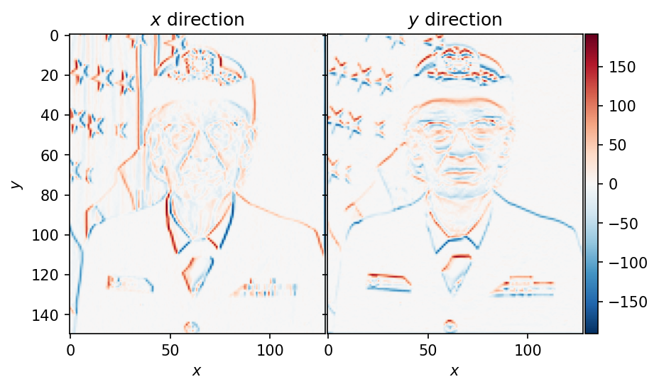
We can see that each derivative image varies depending on each image’s gradient direction.
Check the difference derivative scheme (forward, backward, central)#
Let us check the difference between derivative schemes in the y direction.
[8]:
# compute derivative of images
arr_derivatives = []
vmax = 0
for dmat in [dmat_y, dmat_y_backward, dmat_y_central]:
    arr_derivative = dmat @ arr_image.flatten()
    arr_derivative = arr_derivative.reshape(arr_image.shape)

    # retrieve abosolute maximum value of derivative and choose the largest one
    vmax = val if (val := np.abs(arr_derivative).max()) > vmax else vmax
    arr_derivatives.append(arr_derivative)

fig = plt.figure(dpi=150)
grids = ImageGrid(fig, 111, nrows_ncols=(1, 3), cbar_mode="single")
norm = CenteredNorm(halfrange=vmax)
for ax, arr, title in zip(grids, arr_derivatives, ["forward", "backward", "central"]):  # noqa
    # plot derivative
    im = ax.imshow(arr, cmap="RdBu_r", norm=norm)
    ax.set_xlabel("$x$")
    ax.set_ylabel("$y$")
    ax.set_title(f"{title}")

# plot colorbar
mappable = ScalarMappable(norm=norm, cmap="RdBu_r")
cbar = plt.colorbar(mappable, cax=grids.cbar_axes[0])
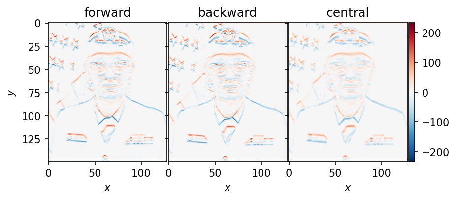
There is no apparent difference between the derivative schemes. The difference seems be more apparent when the gradient is large or the area near the boundary because each scheme has different boundary condition.
Check the difference effect of the laplacian matrix w/ or w/o diagonal neighbors#
[9]:
fig = plt.figure(dpi=150)
grids = ImageGrid(fig, 111, nrows_ncols=(1, 2), cbar_mode="each", axes_pad=0.6, cbar_pad=0.0)
for ax, cax, lmat, title in zip(grids, grids.cbar_axes, [lmat_no_diag, lmat_diag], ["w/o diagonal", "w/ diagonal"]):  # noqa
    # compute laplacian of image
    arr_laplacian = lmat @ arr_image.flatten()
    arr_laplacian = arr_laplacian.reshape(arr_image.shape)

    # plot laplacian of image
    im = ax.imshow(arr_laplacian, cmap="RdBu_r", norm=CenteredNorm())
    ax.set_xlabel("$x$")
    ax.set_ylabel("$y$")
    ax.set_title(f"{title}")

    cbar = plt.colorbar(im, cax=cax)
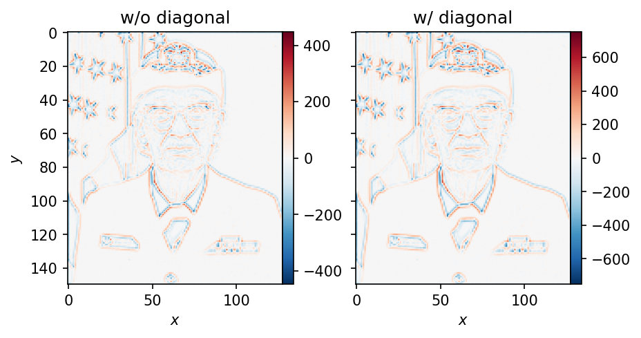
Both laplacian matrices can detect the edge of the image. The laplacian with diagonal neighbors generates larger values than that without diagonal neighbors.
In image processing, the both derivative and laplacian matrices are used for edge detection. In the inversion problem, specific to the tomography, these matrices make a reconstructed image smoother by adding the derivative/laplacian regularization term to the objective function.