Note

This page was generated from notebooks/non-iterative/gcv.ipynb.

GCV criterion

Here we show how to use the Generalized Cross Validation (GCV) criterion to select the optimal regularization parameter for an example ill-posed inverse problem. The definition of the GCV criterion is introduced in this page.

Definition of the example problem

We refer to the famous Fredholm integral equation of the first kind devised by Phillips[1]. Define the function

\[\begin{split}\begin{equation} f(x) \equiv \begin{cases} 1 + \displaystyle\cos\left(\frac{\pi x}{3}\right), & \text{if } | x | < 3, \\ 0, & \text{otherwise} \end{cases}. \end{equation}\end{split}\]

Then, the kernel \(K(s, t)\) and the solution \(x(t)\) are given by

\[\begin{split}\begin{align} K(s, t) &\equiv f(s - t)\\ x(t) &\equiv f(t) \end{align}\end{split}\]

Both integral intervals are \([-6, 6]\).

import numpy as np
from matplotlib import pyplot as plt
from scipy.sparse import diags

from cherab.inversion import GCV, compute_svd
from cherab.inversion.tools import parse_scientific_notation

plt.rcParams["figure.dpi"] = 150

Let us define functions for the kernel, the solution and the right-hand side.

def _func(x: float) -> float:
    if abs(x) < 3.0:
        return 1.0 + np.cos(np.pi * x / 3.0)
    else:
        return 0.0


def kernel(t: float, s: float) -> float:
    """The kernel function."""
    return _func(t - s)


def solution(t: float) -> float:
    """The solution function."""
    return _func(t)

Then we will generate the discretized version of the kernel \(\mathbf{K}\), solution \(\mathbf{x}\) and right-hand side \(\mathbf{b}\) using the trapezoidal rule leading to the following linear system:

\[\begin{equation} \mathbf{K}\mathbf{x} = \mathbf{b}, \end{equation}\]

The size of matrix \(\mathbf{K}\in\mathbb{R}^{M\times N}\) is set to \(M = N = 64\).

s = np.linspace(-6.0, 6.0, num=64, endpoint=True)
t = np.linspace(-6.0, 6.0, num=64, endpoint=True)

# discretize kernel
k_mat = np.zeros((s.size, t.size))
k_mat = np.array([[kernel(i, j) for j in t] for i in s])

# trapezoidal rule
k_mat[:, 0] *= 0.5
k_mat[:, -1] *= 0.5
k_mat *= t[1] - t[0]

# discretize solution
x_t = np.array([solution(i) for i in t])

print(f"{k_mat.shape = }")
print(f"{x_t.shape = }")
print(f"condition number of K is {np.linalg.cond(k_mat):.4g}")

k_mat.shape = (64, 64)
x_t.shape = (64,)
condition number of K is 5.924e+04

The right-hand side \(\mathbf{b}\in\mathbb{R}^{M}\) is usually contaminated by noise. So, we will add a Gaussian noise to the right-hand side.

\[\mathbf{b} = \bar{\mathbf{b}} + \mathbf{e},\]

where \(\bar{\mathbf{b}}\) is the original right-hand side (\(\bar{\mathbf{b}}\equiv \mathbf{K}\mathbf{x}\)), \(\mathbf{e}\) is a vector whose elements are independently sampled from the normal distribution with mean 0 and standard deviation \(10^{-3}\).

b_bar = k_mat @ x_t
rng = np.random.default_rng()
noise = rng.normal(0, 1.0e-3, b_bar.size)
b = b_bar + noise

Solve the inverse problem using the GCV criterion

The solution of the ill-posed linear equation is obtained with the regularization procedure:

\[\begin{equation} \mathbf{x}_\lambda = \left(\mathbf{K}^\mathsf{T}\mathbf{K} + \lambda\mathbf{H}\right)^{-1}\mathbf{K}^\mathsf{T}\mathbf{b}, \end{equation}\]

where \(\mathbf{H}\) is the regularization matrix. Here we set \(\mathbf{H} = \mathbf{D_2}^\mathsf{T}\mathbf{D_2}\), where \(\mathbf{D_2}\) is the second-order difference matrix.

dmat = diags([1, -2, 1], [-1, 0, 1], shape=(t.size, t.size)).tocsr()
print(f"{dmat.shape = }")

dmat.shape = (64, 64)

Then we create GCV solver object after calculating the singular value decomposition according to the series expansion of solution.

hmat = dmat.T @ dmat
s, u, basis = compute_svd(k_mat, hmat)
gcv = GCV(s, u, basis, data=b)

Let us solve the inverse problem.

sol, status = gcv.solve()
print(status)

                    message: ['requested number of basinhopping iterations completed successfully']
                    success: True
                        fun: 1.9460397895292555e-08
                          x: [-2.269e+00]
                        nit: 100
      minimization_failures: 0
                       nfev: 410
                       njev: 205
 lowest_optimization_result:  message: CONVERGENCE: NORM_OF_PROJECTED_GRADIENT_<=_PGTOL
                              success: True
                               status: 0
                                  fun: 1.9460397895292555e-08
                                    x: [-2.269e+00]
                                  nit: 0
                                  jac: [-4.360e-10]
                                 nfev: 2
                                 njev: 1
                             hess_inv: <1x1 LbfgsInvHessProduct with dtype=float64>

Evaluate the GCV criterion

Next we evaluate the solution obtained by the GCV criterion

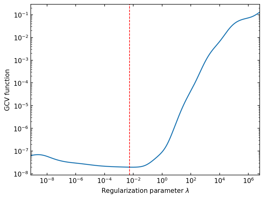
Plot GCV curve

gcv.plot_gcv();

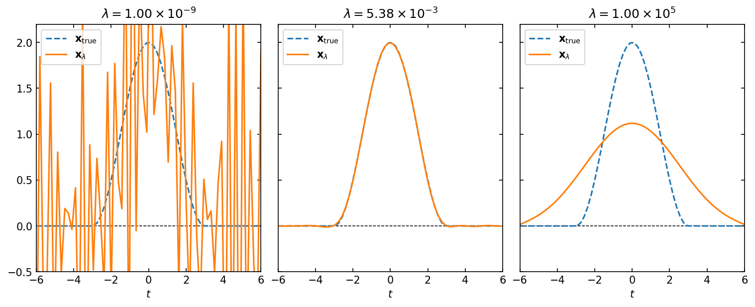
Compare \(\mathbf{x}_\lambda\) with \(\mathbf{x}_\mathrm{true}\)

Let us compare solutions at different regularization parameters \(\lambda=10^{-9}\), \(\lambda_\text{opt}\), \(10^5\) with the true solution \(\mathbf{x}_\mathrm{true}\).

lambdas = [1.0e-9, gcv.lambda_opt, 1.0e5]

fig, axes = plt.subplots(1, 3, figsize=(10, 4), sharey=True, layout="constrained")

for ax, beta in zip(axes, lambdas, strict=False):
    ax.plot(t, x_t, "--", label="$\\mathbf{x}_\\mathrm{true}$")
    ax.plot(t, gcv.solution(beta=beta), label="$\\mathbf{x}_\\lambda$")
    ax.axhline(0, color="black", lw=0.75, ls="--", zorder=-1)

    ax.set_xlim(t.min(), t.max())
    ax.set_ylim(-0.5, x_t.max() * 1.1)
    ax.set_xlabel("$t$")
    parsed_lambda = parse_scientific_notation(f"{beta:.2e}")
    ax.set_title(f"$\\lambda = {parsed_lambda}$")
    ax.tick_params(direction="in", labelsize=10, which="both", top=True, right=True)
    ax.legend(loc="upper left")

Check the relative error

The relative error between the solution \(\mathbf{x}_\lambda\) and the true solution \(\mathbf{x}_\mathrm{true}\) is defined as follows:

\[\begin{equation} \epsilon_\mathrm{rel} = \frac{\|\mathbf{x}_\lambda - \mathbf{x}_\mathrm{true}\|_2}{\|\mathbf{x}_\mathrm{true}\|_2}. \end{equation}\]

Let us seek the minimum \(\epsilon_\mathrm{rel}\) as a function of \(\lambda\).

from scipy.optimize import minimize_scalar

X_T_NORM = np.linalg.norm(x_t, axis=0)


def relative_error(
    log_lambda: float, x_t: np.ndarray = x_t, x_t_norm: float = X_T_NORM, gcv: GCV = gcv
) -> float:
    """Calculate relative error."""
    beta = 10**log_lambda
    sol = gcv.solution(beta=beta)
    return np.linalg.norm(x_t - sol, axis=0) / x_t_norm


# minimize relative error
bounds = gcv.bounds
res = minimize_scalar(
    relative_error,
    bounds=bounds,
    method="bounded",
    args=(x_t, X_T_NORM, gcv),
    options={"xatol": 1.0e-10, "maxiter": 1000},
)

# obtain minimum relative error and lambda
error_min = res.fun
lambda_min = 10**res.x

print(f"minimum relative error: {error_min:.2%} at lambda = {lambda_min:.4g}")

minimum relative error: 0.65% at lambda = 0.008185

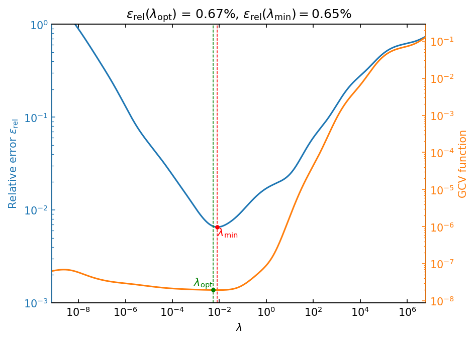
Let us plot the relative error and curvature as a function of \(\lambda\).

# set regularization parameters
num = 500
lambdas = np.logspace(*bounds, num=num)

# calculate errors and gcv
errors = np.asarray([relative_error(log_lambda) for log_lambda in np.linspace(*bounds, num=num)])
gcvs = np.asarray([gcv.gcv(beta) for beta in lambdas])

# create figure
fig, ax1 = plt.subplots()
ax2 = ax1.twinx()

# plot errors and gcv
(p1,) = ax1.loglog(lambdas, errors, color="C0")
(p2,) = ax2.loglog(lambdas, gcvs, color="C1")

# plot minimum error vertical line and point
ax1.axvline(lambda_min, color="r", linestyle="--", linewidth=0.75)
ax1.scatter(lambda_min, error_min, color="r", marker="o", s=10, zorder=2)
ax1.text(
    lambda_min,
    error_min,
    "$\\lambda_\\mathrm{min}$",
    color="r",
    horizontalalignment="left",
    verticalalignment="top",
)

# plot minimum gcv vertical line and point
assert gcv.lambda_opt is not None
min_gcv = gcv.gcv(gcv.lambda_opt)
ax1.axvline(gcv.lambda_opt, color="g", linestyle="--", linewidth=0.75)
ax2.scatter(gcv.lambda_opt, min_gcv, color="g", marker="o", s=10, zorder=2)
ax2.text(
    gcv.lambda_opt,
    min_gcv,
    "$\\lambda_\\mathrm{opt}$",
    color="g",
    horizontalalignment="right",
    verticalalignment="bottom",
)

# set axes
ax1.set(
    xlim=(lambdas[0], lambdas[-1]),
    ylim=(1.0e-3, 1),
    xlabel="$\\lambda$",
    ylabel="Relative error $\\epsilon_\\mathrm{rel}$",
)
ax2.set(ylabel="GCV function")

ax1.yaxis.label.set_color(p1.get_color())
ax2.yaxis.label.set_color(p2.get_color())

ax1.tick_params(axis="x", which="both", direction="in", top=True)
ax1.tick_params(axis="y", which="both", direction="in", colors=p1.get_color())
ax2.tick_params(axis="y", which="both", direction="in", colors=p2.get_color())

ax2.spines["left"].set_color(p1.get_color())
ax2.spines["right"].set_color(p2.get_color())

error_opt = relative_error(np.log10(gcv.lambda_opt))
ax1.set_title(
    f"$\\epsilon_\\mathrm{{rel}}(\\lambda_\\mathrm{{opt}})$ = {error_opt:.2%}, "
    + f"$\\epsilon_\\mathrm{{rel}}(\\lambda_\\mathrm{{min}}) = ${error_min:.2%}"
);

References

[1]

David L Phillips. A technique for the numerical solution of certain integral equations of the first kind. J. ACM, 9(1):84–97, January 1962. doi:10.1145/321105.321114.